Machine Learning & Data Science

Assignments

Assignment 1 — Diabetes Prediction

Task: Predict the onset of diabetes using the Pima Indians Diabetes dataset, with a focus on handling missing values through regression-based imputation, feature engineering, and resampling before training a deep neural network.

Dataset: Pima Indians Diabetes Dataset — 768 samples, 8 features

Method: Regression imputation → Feature engineering → Resampling → DNN

Pipeline Overview

%%{init: {"theme": "base", "themeVariables": {"fontSize": "18px"}, "flowchart": {"padding": 35, "nodeSpacing": 25, "rankSpacing": 40}}}%%
flowchart TD
    A["Raw Data 768×8     "] --> B["Mark Zeros as Missing     "]
    B --> C["Regression Imputation     "]
    C --> D["Feature Eng. + Resample     "]
    D --> E["Train / Val Split     "]
    E --> F["DNN 64→32→16→1     "]
    F --> G["90.04% acc     "]

    style A fill:#E3F2FD,color:#1565C0,stroke:#90CAF9,stroke-width:2px
    style B fill:#F5F5F5,color:#424242,stroke:#BDBDBD,stroke-width:2px
    style C fill:#FFF3E0,color:#E65100,stroke:#FFCC80,stroke-width:2px
    style D fill:#F3E5F5,color:#6A1B9A,stroke:#CE93D8,stroke-width:2px
    style E fill:#F5F5F5,color:#424242,stroke:#BDBDBD,stroke-width:2px
    style F fill:#E3F2FD,color:#1565C0,stroke:#90CAF9,stroke-width:2px
    style G fill:#E8F5E9,color:#2E7D32,stroke:#A5D6A7,stroke-width:2px

Pipeline Description: The raw data contains “zero values” in columns such as Glucose and BMI, which actually represent missing data. Linear regression is used to impute each column sequentially, followed by feature engineering and resampling to balance positive and negative samples. Finally, a 4-layer DNN performs binary classification, improving from a baseline of 74% to 90.04%.

Exploratory Data Analysis

Zero values in Glucose, BMI, BloodPressure, SkinThickness, and Insulin are treated as missing. After removing rows with missing values, 336 clean rows remain for fitting imputation models.

Feature Correlation Matrix (after removing rows with NaN)

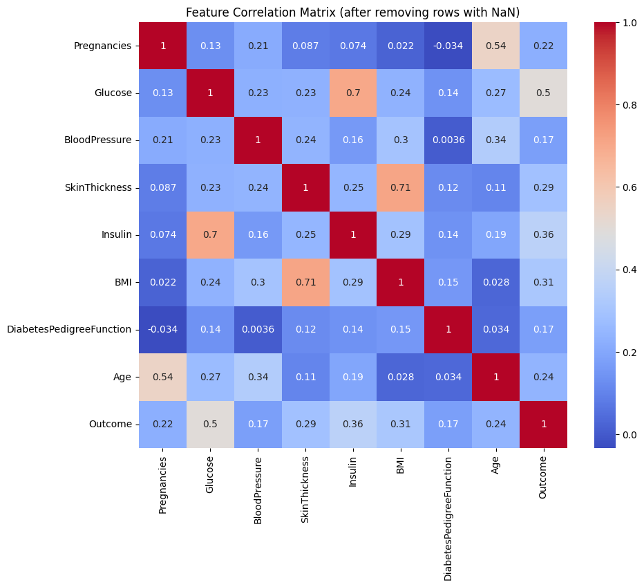
Key Observations: Glucose → Outcome has a correlation of 0.50, making it the strongest predictor for diabetes; SkinThickness ↔︎ BMI reaches 0.71, allowing BMI to impute SkinThickness; Insulin ↔︎ Glucose reaches 0.70, allowing Glucose to impute Insulin; Age ↔︎ Pregnancies is 0.54, consistent with biological expectations.

Missing Value Imputation

%%{init: {"theme": "base", "themeVariables": {"fontSize": "18px"}, "flowchart": {"padding": 35}}}%%
flowchart TD
    A["Outcome     "]
    B["Glucose     "]
    C["BMI     "]
    D["Insulin     "]
    E["SkinThickness     "]
    F["Age     "]
    G["BloodPressure     "]

    A -->|"predicts"| B
    B -->|"predicts"| C
    B -->|"predicts"| D
    C -->|"predicts"| E
    B -->|"predicts"| E
    F -->|"predicts"| G
    C -->|"predicts"| G

    style A fill:#FFF3E0,color:#E65100,stroke:#FFCC80,stroke-width:2px
    style B fill:#E3F2FD,color:#1565C0,stroke:#90CAF9,stroke-width:2px
    style C fill:#E8F5E9,color:#2E7D32,stroke:#A5D6A7,stroke-width:2px
    style D fill:#FCE4EC,color:#C62828,stroke:#F48FB1,stroke-width:2px
    style E fill:#F3E5F5,color:#6A1B9A,stroke:#CE93D8,stroke-width:2px
    style F fill:#FFF3E0,color:#E65100,stroke:#FFCC80,stroke-width:2px
    style G fill:#E0F2F1,color:#00695C,stroke:#80CBC4,stroke-width:2px

Imputation Order: Using the most highly correlated known columns as independent variables, linear regression is applied sequentially: Outcome → Glucose → BMI → Insulin / SkinThickness → BloodPressure. Each step uses only columns that already exist or have already been imputed as predictors.

# Fill Glucose using Outcome
X_train = df_non_missing[['Outcome']]
y_train = df_non_missing['Glucose']
model = LinearRegression()
model.fit(X_train, y_train)

# Fill BMI using Glucose
X_train = df_non_missing[['Glucose']]
y_train = df_non_missing['BMI']

# Fill Insulin using BMI + Glucose
X_train = df_non_missing[['BMI', 'Glucose']]
y_train = df_non_missing['Insulin']

# Fill BloodPressure using Age + BMI
X_train = df_non_missing[['Age', 'BMI']]
y_train = df_non_missing['BloodPressure']

Model Architecture

%%{init: {"theme": "base", "themeVariables": {"fontSize": "18px"}, "flowchart": {"padding": 35}}}%%
flowchart LR
    I["Input 8+ feat     "] --> L1["Dense 64 ReLU     "] --> L2["Dense 32 ReLU     "] --> L3["Dense 16 ReLU     "] --> O["Dense 1 Sigmoid     "]

    style I  fill:#E3F2FD,color:#1565C0,stroke:#90CAF9,stroke-width:2px
    style L1 fill:#E3F2FD,color:#1565C0,stroke:#90CAF9,stroke-width:2px
    style L2 fill:#E3F2FD,color:#1565C0,stroke:#90CAF9,stroke-width:2px
    style L3 fill:#E3F2FD,color:#1565C0,stroke:#90CAF9,stroke-width:2px
    style O  fill:#E8F5E9,color:#2E7D32,stroke:#A5D6A7,stroke-width:2px

model = Sequential()
model.add(Dense(64, input_dim=X_train.shape[1], activation='relu'))
model.add(Dense(32, activation='relu'))
model.add(Dense(16, activation='relu'))
model.add(Dense(1, activation='sigmoid'))

Training Setup

model.compile(
    loss='binary_crossentropy',
    optimizer='adam',
    metrics=['accuracy']
)
model.fit(X_train, y_train, epochs=10, batch_size=32, validation_split=0.2)

Results

Metric	Value
Baseline accuracy (no imputation)	74.03%
Final accuracy (with imputation + feature engineering + resampling)	90.04%
Improvement	+16.01 pp

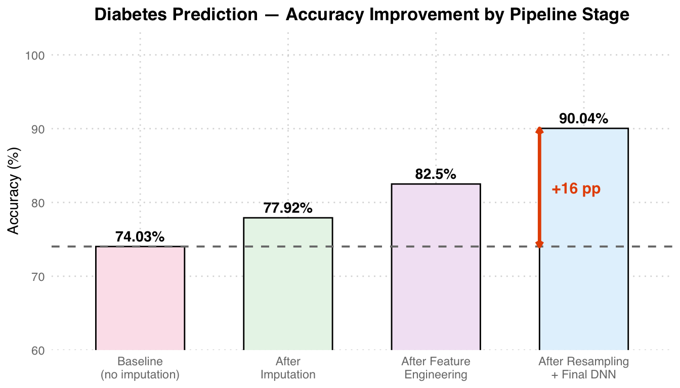
Accuracy Analysis: The baseline (directly dropping missing values) achieves only 74.03%. After regression imputation, accuracy increases to 77.92%, feature engineering adds ~5 pp, and finally resampling + DNN reaches 90.04%, a total improvement of +16 pp. The grey dashed line marks the baseline reference, and the orange arrow indicates the overall gain.

---

Assignment 2 — US Wildfire Analysis

Task: Analyze 1.88 million US wildfire records to model annual frequency trends using Poisson regression, and predict wildfire causes using a multi-layer perceptron.

Dataset: US Wildfires (1992–2015) — 1,880,465 records, Kaggle

Method: Poisson Regression (trend analysis) + MLP (cause classification)

Poisson Regression

Models the annual count of wildfires as a function of year to estimate the long-term trend.

import statsmodels.api as sm
import statsmodels.formula.api as smf

poisson_model = smf.glm(
    formula='Count ~ FIRE_YEAR',
    data=fire_counts,
    family=sm.families.Poisson()
).fit()

print(poisson_model.summary())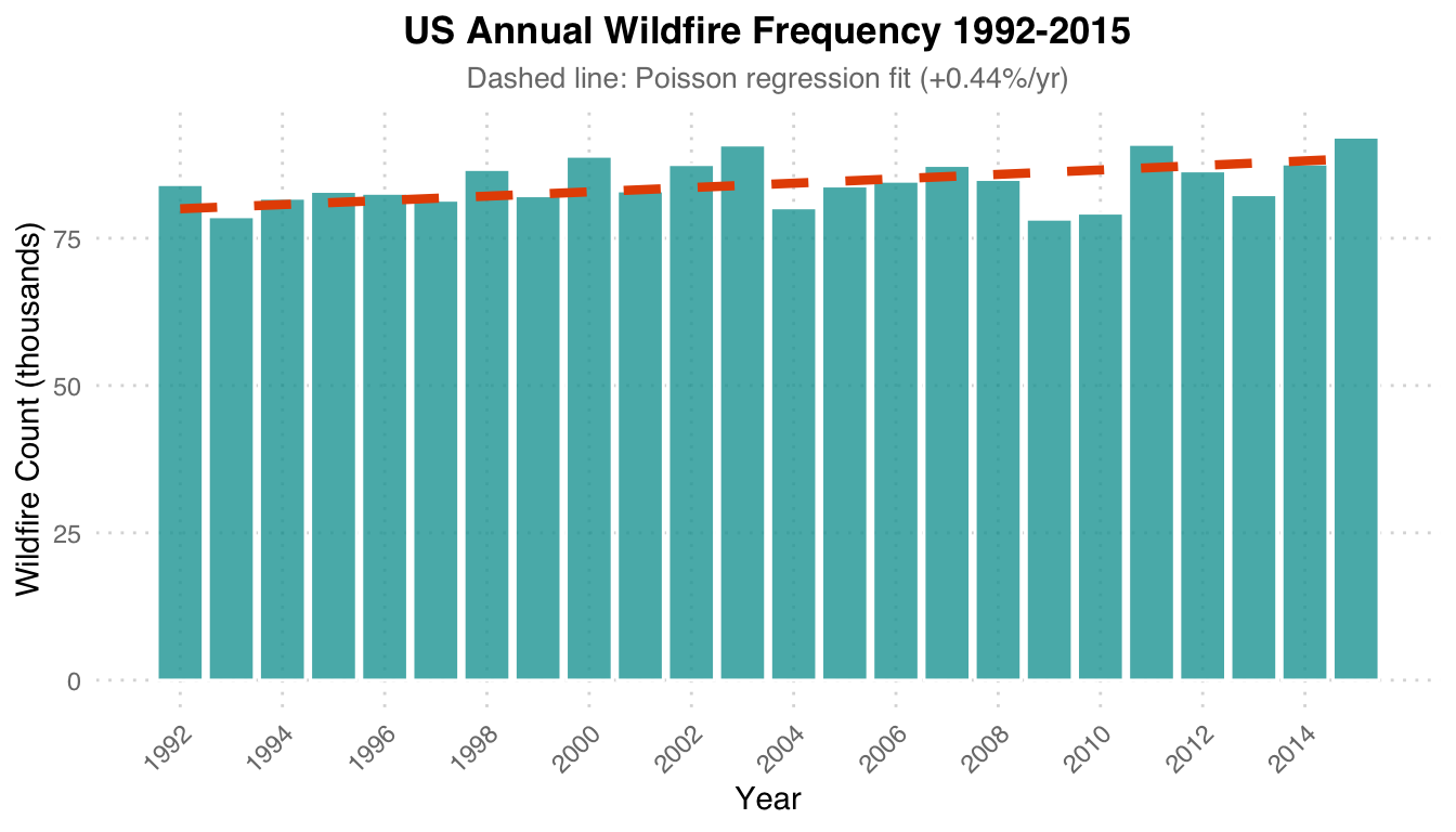

Poisson Trend: A Poisson regression fitted with year as the independent variable estimates that annual wildfire frequency increases at a rate of +0.44% per year. The orange dashed line is the regression fit, and the teal bars represent the actual counts for each year.

MLP Model Architecture

Features: FIRE_SIZE, LATITUDE, LONGITUDE, FIRE_YEAR, MONTH

%%{init: {"theme": "base", "themeVariables": {"fontSize": "18px"}, "flowchart": {"padding": 35}}}%%
flowchart LR
    F["5 Features     "] --> D1["Dense 64 ReLU     "] --> DR1["Dropout 0.3     "] --> D2["Dense 64 ReLU     "] --> DR2["Dropout 0.3     "] --> O["Softmax → N cls     "]

    style F   fill:#E3F2FD,color:#1565C0,stroke:#90CAF9,stroke-width:2px
    style D1  fill:#E3F2FD,color:#1565C0,stroke:#90CAF9,stroke-width:2px
    style DR1 fill:#FFF3E0,color:#E65100,stroke:#FFCC80,stroke-width:2px
    style D2  fill:#E3F2FD,color:#1565C0,stroke:#90CAF9,stroke-width:2px
    style DR2 fill:#FFF3E0,color:#E65100,stroke:#FFCC80,stroke-width:2px
    style O   fill:#E8F5E9,color:#2E7D32,stroke:#A5D6A7,stroke-width:2px

Architecture Description: A simple MLP with two Dense 64 layers + Dropout 0.3. Blue = Dense layers, Orange = Dropout regularization, Green = Softmax output (10 wildfire cause classes).

model = Sequential()
model.add(Dense(64, input_dim=X_train.shape[1], activation='relu'))
model.add(Dropout(0.3))
model.add(Dense(64, activation='relu'))
model.add(Dropout(0.3))
model.add(Dense(num_classes, activation='softmax'))

model.compile(
    loss='categorical_crossentropy',
    optimizer='adam',
    metrics=['accuracy']
)

Training Setup

model.fit(X_train, y_train, epochs=20, batch_size=32, validation_split=0.2)
# Train/Test Split: 70/30

Results

Metric	Value
Wildfire cause prediction accuracy	~45.6%
Poisson regression trend	+0.44% annual increase
Total records processed	1,880,465

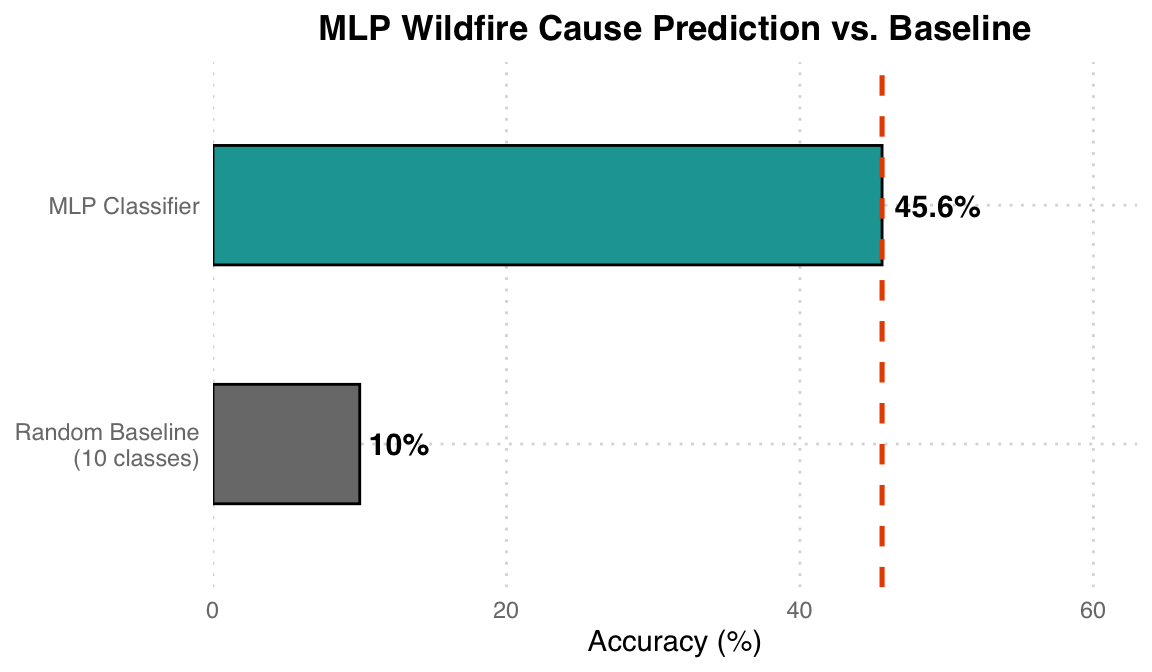
Results Analysis: The 10-class random guess baseline is 10%, while the MLP achieves ~45.6%, far better than random but still with room for improvement. The relatively low classification accuracy reflects the inherent difficulty of determining wildfire causes based solely on geographic location (latitude/longitude) and time (year, month) – many causes (human vs. lightning) overlap significantly in spatial distribution.

---

Final Project — Cervical Cancer Screening

Task: Classify cervical cell images into three types (Type 1, 2, 3) corresponding to different levels of cervical transformation zone, using transfer learning with EfficientNet-B7 and Focal Loss to handle class imbalance.

Dataset: Intel & MobileODT Cervical Cancer Screening (Kaggle) — 3-class image classification

Method: EfficientNet-B7 (ImageNet pretrained, fine-tuned) + Focal Loss + Data Augmentation

Transfer Learning Strategy

%%{init: {"theme": "base", "themeVariables": {"fontSize": "18px"}, "flowchart": {"padding": 35}}}%%
flowchart LR
    A["Pretrained EfficientNet-B7     "] --> B["Freeze Backbone     "] --> C["Classifier → 3 cls     "] --> D["Focal Loss γ=2     "] --> E["Type 1/2/3     "]

    style A fill:#E3F2FD,color:#1565C0,stroke:#90CAF9,stroke-width:2px
    style B fill:#F5F5F5,color:#424242,stroke:#BDBDBD,stroke-width:2px
    style C fill:#FFF3E0,color:#E65100,stroke:#FFCC80,stroke-width:2px
    style D fill:#F3E5F5,color:#6A1B9A,stroke:#CE93D8,stroke-width:2px
    style E fill:#E8F5E9,color:#2E7D32,stroke:#A5D6A7,stroke-width:2px

Transfer Learning Strategy: The ImageNet-pretrained EfficientNet-B7 backbone is first frozen as a feature extractor, and only the newly added classification head is trained. Focal Loss is used to address the sample imbalance among Type 1/2/3.

Model Architecture

from torchvision.models import efficientnet_b7, EfficientNet_B7_Weights

model = efficientnet_b7(weights=EfficientNet_B7_Weights.IMAGENET1K_V1)
num_features = model.classifier[1].in_features
model.classifier[1] = nn.Linear(num_features, num_classes)  # num_classes = 3
model = model.to(device)

Focal Loss Implementation

Focal Loss down-weights easy examples and focuses training on hard, misclassified samples – especially useful for imbalanced class distributions.

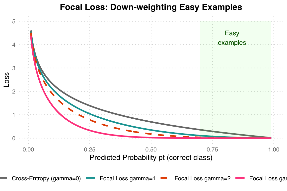
Focal Loss Principle: When gamma=0, it is equivalent to standard Cross-Entropy. The larger the gamma, the less penalty is applied to “already correctly classified easy examples” (the green region on the right), allowing the model to focus on learning hard examples. This project uses gamma=2 (orange dashed line).

class FocalLoss(nn.Module):
    def __init__(self, alpha=1, gamma=2, reduction="mean"):
        super(FocalLoss, self).__init__()
        self.alpha = alpha
        self.gamma = gamma
        self.reduction = reduction

    def forward(self, inputs, targets):
        ce_loss = nn.CrossEntropyLoss(reduction="none")(inputs, targets)
        pt = torch.exp(-ce_loss)
        focal_loss = self.alpha * (1 - pt) ** self.gamma * ce_loss
        if self.reduction == "mean":
            return focal_loss.mean()
        elif self.reduction == "sum":
            return focal_loss.sum()
        return focal_loss

criterion = FocalLoss(alpha=1, gamma=2)

Training Setup

optimizer = optim.Adam(model.parameters(), lr=0.001)
num_epochs = 20
batch_size = 32

for epoch in range(num_epochs):
    model.train()
    for inputs, labels in train_loader:
        inputs, labels = inputs.to(device), labels.to(device)
        optimizer.zero_grad()
        outputs = model(inputs)
        loss = criterion(outputs, labels)
        loss.backward()
        optimizer.step()

Results

Class	Description	Accuracy
Type 1	Ectocervix (fully visible transformation zone)	87.5%
Type 2	Partially visible transformation zone	92.3%
Type 3	Endocervix (transformation zone not visible)	78.5%

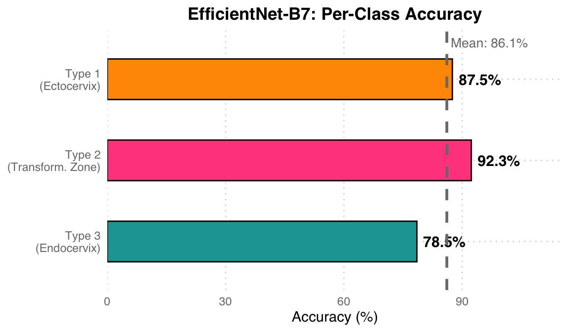
Classification Results Analysis: Type 2 (partially visible transformation zone) achieves the highest accuracy at 92.3% due to its most distinctive features. Type 3 (transformation zone not visible) has the lowest at 78.5%, as it lacks identifiable surface structural features, making classification the most difficult. The mean accuracy is 86.1% (grey dashed line). Focal Loss effectively improved the learning performance on minority classes.