%%{init: {"theme": "base", "themeVariables": {"fontSize": "18px"}, "flowchart": {"padding": 35}}}%%
flowchart TD
    A["Load Image 1546×1029×3     "] --> B["Split R, G, B     "]
    B --> C["np.linalg.svd per channel     "]
    C --> D["Reconstruct A_k for k = 1..1029     "]
    D --> E["Compute MSE, PSNR, 2-norm     "]
    E --> F["Compare 2-norm vs σ_k+1     "]

    style A fill:#E3F2FD,color:#1565C0,stroke:#90CAF9,stroke-width:2px
    style B fill:#F5F5F5,color:#424242,stroke:#BDBDBD,stroke-width:2px
    style C fill:#FFF3E0,color:#E65100,stroke:#FFCC80,stroke-width:2px
    style D fill:#F3E5F5,color:#6A1B9A,stroke:#CE93D8,stroke-width:2px
    style E fill:#E3F2FD,color:#1565C0,stroke:#90CAF9,stroke-width:2px
    style F fill:#E8F5E9,color:#2E7D32,stroke:#A5D6A7,stroke-width:2px
Data Analysis Mathematics
Data Analysis Mathematics · National Chung Hsing University, Graduate Institute of Data Science and Information Computing
Assignments
HW1 — SVD Image Compression
Topic: Verify the Eckart-Young theorem using SVD decomposition: \(\|A - A_k\|_2 = \sigma_{k+1}\)
Dataset: Color photo 1546×1029 pixels (RGB three channels)
Pipeline Overview
Method Description: The photo is treated as matrix A, and SVD is performed separately on each of the RGB channels. We deliberately avoid using np.linalg.norm(ord=2) (since its internal implementation relies on SVD, which would create circular reasoning), and instead use a Monte Carlo random vector method to approximate the operator 2-norm, then compare its trend with σ_{k+1}.
Key Formulas
SVD Decomposition:
\[A = U \Sigma V^T, \quad A_k = \sum_{i=1}^{k} \sigma_i u_i v_i^T\]
Eckart-Young Theorem:
\[\|A - A_k\|_2 = \sigma_{k+1}\]
Results
| k | 2-norm (approx) | σ_{k+1} | MSE | PSNR (dB) |
|---|---|---|---|---|
| 1 | 3,310 | 34,072 | 3,363 | 12.95 |
| 10 | 1,556 | 10,116 | 1,403 | 16.77 |
| 50 | 837 | 3,645 | 487 | 21.35 |
| 100 | 577 | 2,108 | 241 | 24.37 |
| 300 | 234 | 699 | 42 | 31.88 |
| 500 | 116 | 340 | 10 | 38.04 |
| 700 | 54 | 172 | 2.2 | 44.70 |
Reconstruction Quality
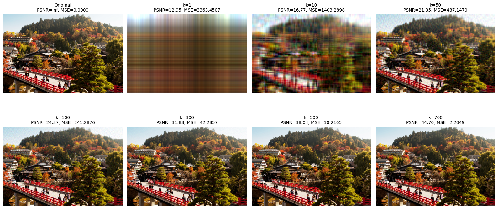
Visualization: At k=1, the original image is barely recognizable; at k=50, the main contours become distinguishable; above k=300, the result closely resembles the original. At k=507 (bottom right), PSNR reaches 38 dB, making differences from the original virtually imperceptible to the human eye.
MSE / PSNR / 2-norm Analysis
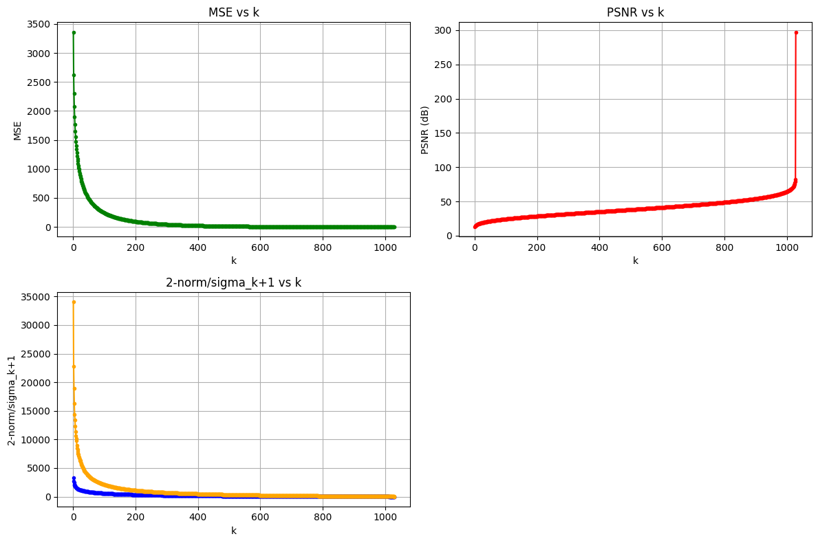
Conclusion: MSE decreases and PSNR increases as k grows, and the 2-norm follows the same decreasing trend as σ_{k+1}, indirectly verifying the Eckart-Young theorem. The Monte Carlo method underestimates the true 2-norm due to random sampling, but the overall trend remains consistent.
HW2 — Handwritten Digit Recognition
Topic: Comparing 8 classification methods on the USPS handwritten digit dataset
Dataset: USPS handwritten digits (16×16 grayscale, 10 classes for digits 0-9)
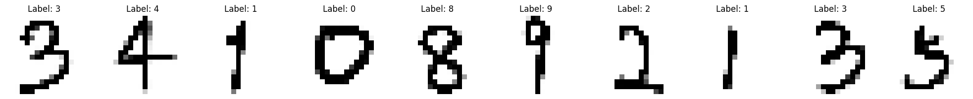
Dataset Samples
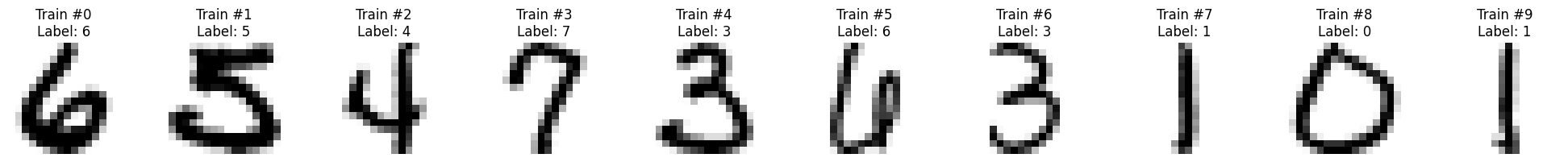
Data Characteristics: Each image is only 16×16 = 256 pixels, an extremely low resolution that still preserves the basic structure of digits. This allows matrix decomposition methods (SVD / HOSVD) to effectively capture low-dimensional features.
Methods Overview
| Category | Method | Description |
|---|---|---|
| Baseline | Mean Method | Compute the mean image for each class and classify by Euclidean distance |
| Enhanced Mean | Iterative refinement considering inter-class confusion patterns | |
| Matrix Decomposition | SVD (k=20) | Build SVD basis for each class and classify by projection residual |
| HOSVD | Tucker decomposition (tensorly), rank (10,10,20) | |
| Traditional ML | SVM | sklearn SVC |
| KNN | sklearn KNeighborsClassifier | |
| Random Forest | sklearn RandomForestClassifier | |
| Deep Learning | CNN (PyTorch) | Conv2D → MaxPool → Dense, 50 epochs |
Accuracy Comparison
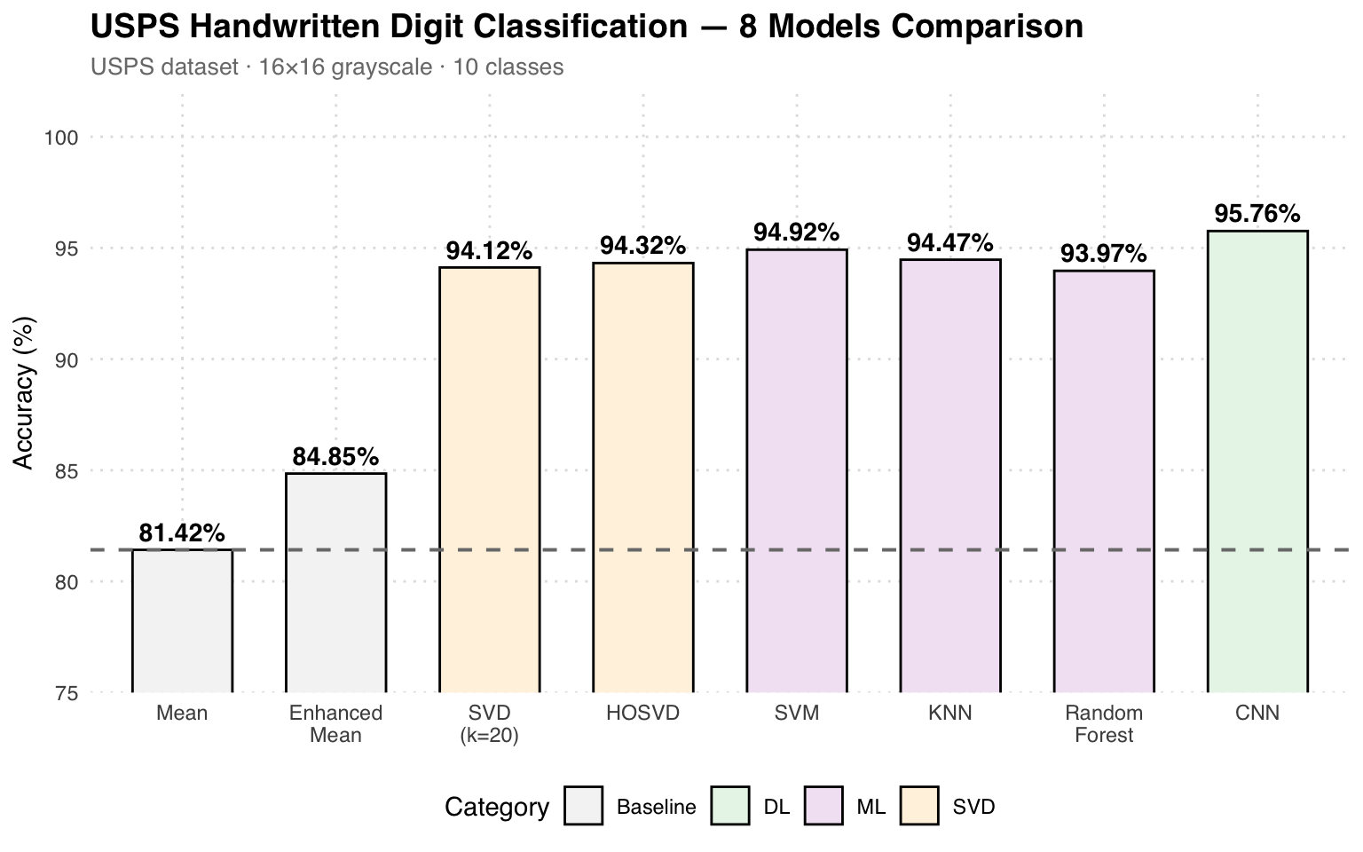
Results Analysis: The Mean method achieves only 81.42% as a baseline. SVD (k=20) jumps to 94.12%, demonstrating that low-rank approximation effectively captures digit structure. Traditional ML (SVM at 94.92%) performs similarly to the SVD family. CNN wins at 95.76%, but its training time is 98 seconds, far higher than KNN’s 0.45 seconds.
Training Time Comparison
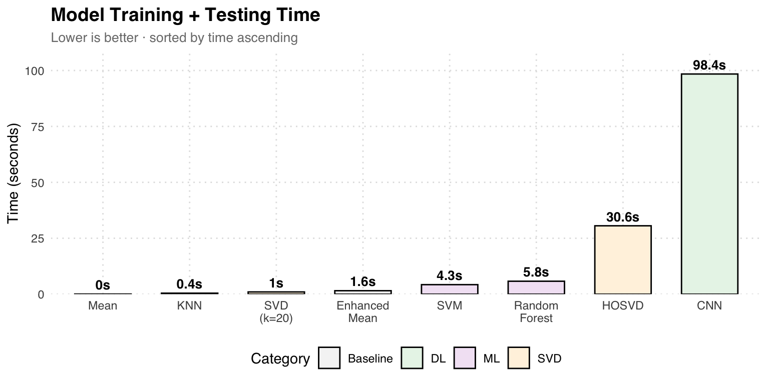
Speed vs Accuracy: KNN achieves 94.47% in just 0.45 seconds, making it the most cost-effective model. CNN is the most accurate (95.76%) but takes 98 seconds. HOSVD (Tucker decomposition) achieves similar accuracy to SVD but is 30 times slower.
SVD Confusion Matrix
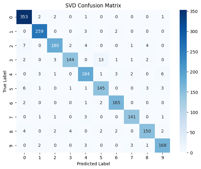
Confusion Matrix Analysis: The SVD method performs best on digits 0 and 1 (353/264 correct), while confusion is higher for digits 3 and 7 (13 misclassifications of 3 as 5). The overall 94.12% accuracy is excellent for a training-free matrix decomposition method.
Misclassified Samples
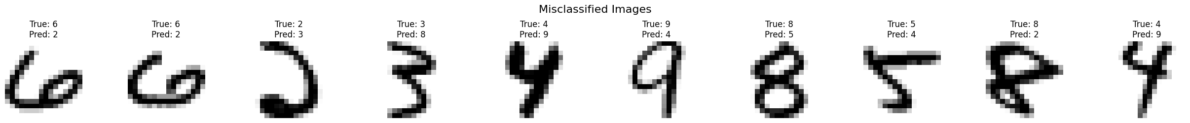
Misclassification Analysis: These samples are difficult to identify even for the human eye. For example, True: 6 is predicted as 2 (similar curved strokes), and True: 3 is predicted as 8 (similar shapes). At the low resolution of 16×16, the structural differences between some digits are extremely small.
Real Handwriting Test
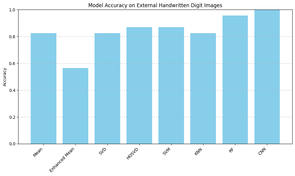
External Validation: All models were tested using handwritten digit photos taken with a phone. CNN achieves 100% perfect recognition, Random Forest 95%, while Enhanced Mean only 56%. This confirms that deep learning has the strongest generalization ability for real-world handwriting variations.