GIS & Python Programming

Assignments

Lab 2 — Retirement Calculator

Topic: A financial-planning tool built on compound-interest calculations.

Key Concepts: Functions, loops, formatted output, compound interest

%%{init: {"theme": "base", "themeVariables": {"fontSize": "18px"}, "flowchart": {"padding": 35}}}%%
flowchart LR
    A["User Input     "] --> B["Monthly Contribution     "] --> C["Compound Interest     "] --> D["Year-by-Year Projection     "] --> E["Millionaire Calculator     "]

    style A fill:#E3F2FD,color:#1565C0,stroke:#90CAF9,stroke-width:2px
    style B fill:#F5F5F5,color:#424242,stroke:#BDBDBD,stroke-width:2px
    style C fill:#FFF3E0,color:#E65100,stroke:#FFCC80,stroke-width:2px
    style D fill:#E8F5E9,color:#2E7D32,stroke:#A5D6A7,stroke-width:2px
    style E fill:#E8F5E9,color:#2E7D32,stroke:#A5D6A7,stroke-width:2px

Three modes: (1) Year-by-year fund projection (monthly compounding), (2) Millionaire calculator (years until $1M), (3) Interest-rate comparison table (1–30% annual). Example: $500/month at 10% annual return for 30 years → $1.14M.

# Year-by-year retirement fund projection
def calculate_fund(monthly, rate, years):
    balance = 0
    monthly_rate = rate / 12
    for year in range(1, years + 1):
        for month in range(12):
            balance += monthly
            balance *= (1 + monthly_rate)
        print(f"Year {year:3d}: ${balance:>12,.2f}")
    return balance

# Millionaire Calculator
def years_to_million(monthly, rate):
    balance, months = 0, 0
    monthly_rate = rate / 12
    while balance < 1_000_000:
        balance += monthly
        balance *= (1 + monthly_rate)
        months += 1
    return months // 12, months % 12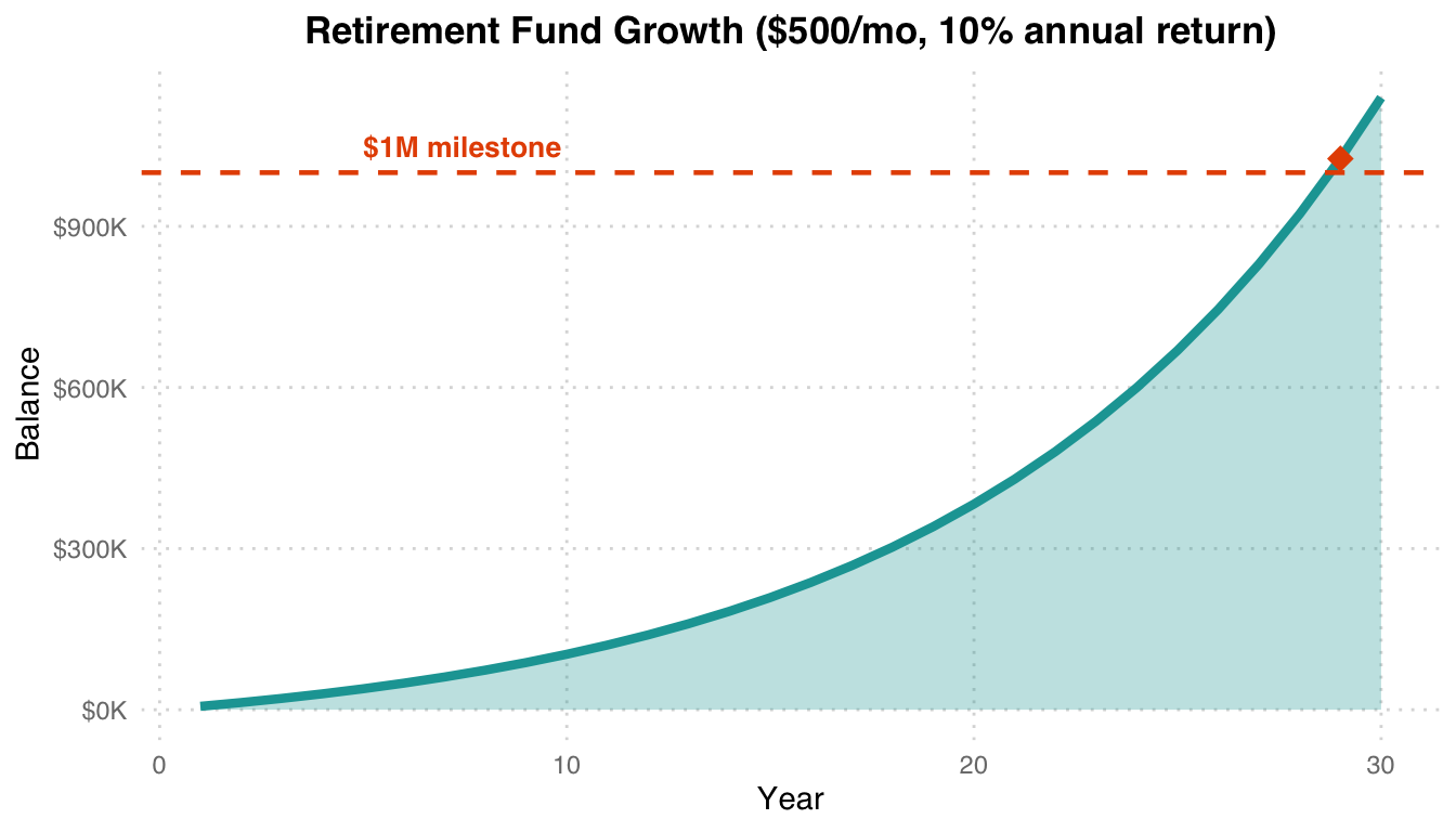

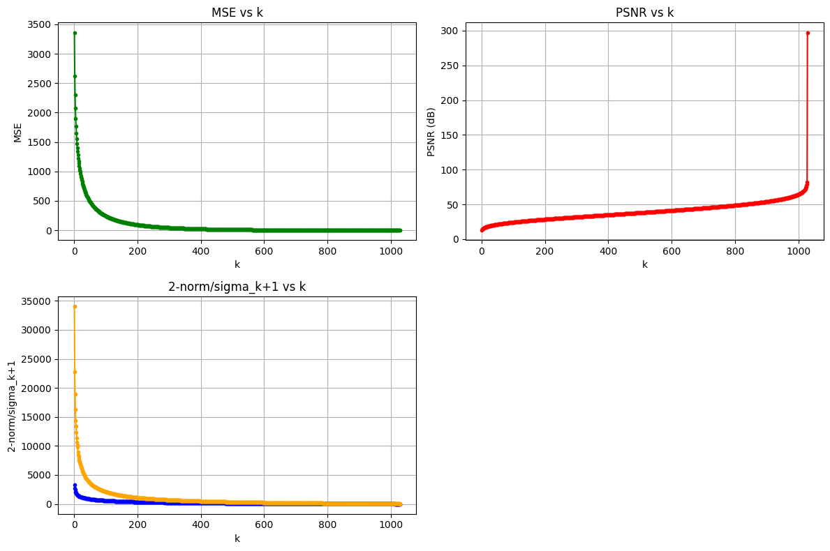
Compound interest effect: Slow growth in the first 15 years, exponential acceleration in the next 15. $500/month at 10% annual return reaches $1M in roughly 21 years (orange diamond). Compounding is the core driver of long-term investing.

---

Lab 3 — Gradebook Manager

Topic: Interactive student grade management with full CRUD operations.

Key Concepts: Lists, nested data structures, menu-driven programming, input validation

# Menu-driven gradebook
def main_menu():
    while True:
        print("\n1. Add student")
        print("2. Remove student")
        print("3. Modify grade")
        print("4. Display gradebook")
        print("5. Find highest/lowest")
        print("6. Exit")
        choice = input("Select: ")
        # ... handle each option

Design highlights: Stores student records as a nested list [name, grade] and uses a while loop to drive a persistent interactive menu. Includes input validation (grades 0–100) and error handling.

---

Lab 4 — Modules, Functions & OOP

Topic: Modular programming, reusable modules, and object-oriented design.

Key Concepts: Module imports, OOP (classes), CSV I/O, distance calculations

%%{init: {"theme": "base", "themeVariables": {"fontSize": "18px"}, "flowchart": {"padding": 35}}}%%
flowchart TD
    A["Lab 4 Modules     "] --> B["(a) CSV Field Counter     "]
    A --> C["(b) Parcel Tax Calculator     "]
    A --> D["(c) Distance Calculator     "]

    B --> B1["mycount.py + callingscript.py     "]
    C --> C1["parcelclass.py → OOP     "]
    D --> D1["Euclidean + Great Circle     "]

    style A fill:#E3F2FD,color:#1565C0,stroke:#90CAF9,stroke-width:2px
    style B fill:#FFF3E0,color:#E65100,stroke:#FFCC80,stroke-width:2px
    style C fill:#E8F5E9,color:#2E7D32,stroke:#A5D6A7,stroke-width:2px
    style D fill:#F3E5F5,color:#6A1B9A,stroke:#CE93D8,stroke-width:2px
    style B1 fill:#F5F5F5,color:#424242,stroke:#BDBDBD,stroke-width:2px
    style C1 fill:#F5F5F5,color:#424242,stroke:#BDBDBD,stroke-width:2px
    style D1 fill:#F5F5F5,color:#424242,stroke:#BDBDBD,stroke-width:2px

# (b) Parcel class with tax assessment
class Parcel:
    def __init__(self, parcel_id, land_use, market_value):
        self.parcel_id = parcel_id
        self.land_use = land_use
        self.market_value = market_value

    def assess_tax(self):
        rates = {"SFR": 0.05, "MFR": 0.04}
        rate = rates.get(self.land_use, 0.02)
        return self.market_value * rate

# (c) Great Circle Distance (Haversine formula)
import math
def great_circle(lat1, lon1, lat2, lon2):
    R = 6371  # Earth radius in km
    dlat = math.radians(lat2 - lat1)
    dlon = math.radians(lon2 - lon1)
    a = (math.sin(dlat/2)**2 +
         math.cos(math.radians(lat1)) *
         math.cos(math.radians(lat2)) *
         math.sin(dlon/2)**2)
    return R * 2 * math.asin(math.sqrt(a))

Three sub-tasks: (a) Count empty values per column in a CSV file, (b) Use OOP to build a Parcel class that assesses property tax (SFR 5%, MFR 4%, others 2%), (c) Compute the great-circle distance between two points on Earth using the Haversine formula.

---

Lab 5 — Pandas Data Analysis

Topic: DataFrame manipulation, grouping, pivoting, and multi-dataset merging.

Datasets: MovieLens (100K ratings), COVID-19 global time series

Key Concepts: pandas Series/DataFrame, boolean indexing, GroupBy, pivot tables, merge/join

# COVID-19 fatality rate analysis
fatality = (deaths_total / confirmed_total * 100).sort_values(ascending=False)
# Peru: 9.17%, Mexico: 7.58%, South Africa: 2.68%

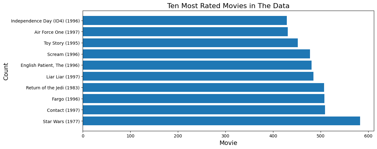
# MovieLens: most rated movies
top_movies = ratings.groupby('movieId').size().sort_values(ascending=False).head(10)

# Multi-DataFrame merge
merged = pd.merge(users, ratings, on='userId')
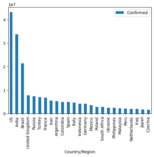
merged = pd.merge(merged, movies, on='movieId')

Analysis highlights: (1) MovieLens — identifying the most-rated movies and the films with the largest male/female rating gap; (2) COVID-19 — top-25 countries by confirmed cases, fatality-rate ranking (Peru highest at 9.17%), and monthly increment analysis (the US gained +4.3M cases in September 2021).

---

Lab 6 — Data Visualization

Topic: Publication-quality charts with matplotlib and interactive plots with Altair.

Datasets: MovieLens, COVID-19, Seattle weather (Vega)

Top 10 Most-Reviewed Movies

COVID-19 Top 25 Countries

Gender Rating Differences

Seattle Weather Distribution

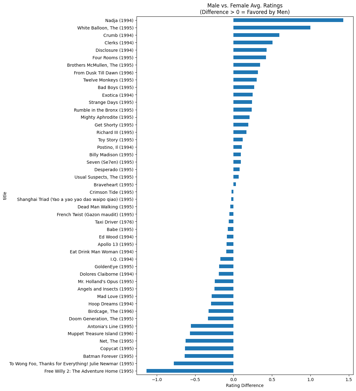
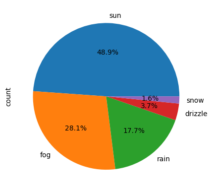
Visualization techniques: Horizontal bar charts to compare review counts, scatter plots to expose male/female rating differences, pie charts for weather-type distribution, and line charts to track COVID-19 trends. The Altair section also produced an interactive linked chart (click a country → reveal its death-trend curve).

---

Lab 7 — GUI Development with PyQt5

Topic: Building a desktop number-guessing game with a graphical interface.

Key Concepts: PyQt5 widgets, event-driven programming, signal/slot, Qt Designer

%%{init: {"theme": "base", "themeVariables": {"fontSize": "18px"}, "flowchart": {"padding": 35}}}%%
flowchart LR
    A["Qt Designer     "] --> B["frmGuess.py     "] --> C["lab7.py     "] --> D["Number Game GUI     "]

    style A fill:#F5F5F5,color:#424242,stroke:#BDBDBD,stroke-width:2px
    style B fill:#E3F2FD,color:#1565C0,stroke:#90CAF9,stroke-width:2px
    style C fill:#FFF3E0,color:#E65100,stroke:#FFCC80,stroke-width:2px
    style D fill:#E8F5E9,color:#2E7D32,stroke:#A5D6A7,stroke-width:2px

# Number guessing game with hint system
class GuessGame:
    def __init__(self):
        self.target = random.randint(1, 100)
        self.guesses = 0

    def make_guess(self, n):
        self.guesses += 1
        if n == self.target:
            return "Correct!"
        return "Higher!" if n < self.target else "Lower!"

    def use_hint(self):
        """Costs 5 guesses, reveals number within ±5"""
        self.guesses += 5
        return (self.target - 5, self.target + 5)

GUI features: A 1–100 random-number guessing game with (1) guess tracking, (2) a hint system that costs 5 guesses and narrows the target window to ±5, and (3) win detection plus reset. The interface is laid out in Qt Designer; frmGuess.py is the auto-generated UI code.

---

Lab 8 — ArcGIS API for Python

Topic: Programmatic map creation and spatial-data querying with ArcGIS Online.

Key Concepts: ArcGIS authentication, WebMap, FeatureLayer queries, basemap cycling

from arcgis.gis import GIS
from arcgis.mapping import WebMap

gis = GIS("https://www.arcgis.com", username, password)
m = gis.map("University of Texas at Dallas", zoomlevel=15)

# Search and add feature layers
items = gis.content.search("UTD Buildings", item_type="Feature Layer")
m.add_layer(items[0])

# Query building attributes
fl = items[0].layers[0]
fl.properties.fields  # Inspect field schema

GIS operations: Connect to ArcGIS Online via the Python API, build an interactive map centered on the UTD campus, search for and overlay building layers, inspect attribute-field schemas, and cycle through different basemap styles.

---

Lab 10 — Web Scraping & APIs

Topic: Extracting data from web sources using APIs and scraping tools.

Key Concepts: requests, JSON parsing, BeautifulSoup (HTML), Selenium (dynamic content)

%%{init: {"theme": "base", "themeVariables": {"fontSize": "18px"}, "flowchart": {"padding": 35}}}%%
flowchart LR
    A["requests GET     "] --> B["JSON / HTML     "]
    B --> C["BeautifulSoup     "]
    B --> D["json.loads()     "]
    C --> E["Structured Data     "]
    D --> E

    style A fill:#E3F2FD,color:#1565C0,stroke:#90CAF9,stroke-width:2px
    style B fill:#F5F5F5,color:#424242,stroke:#BDBDBD,stroke-width:2px
    style C fill:#FFF3E0,color:#E65100,stroke:#FFCC80,stroke-width:2px
    style D fill:#E8F5E9,color:#2E7D32,stroke:#A5D6A7,stroke-width:2px
    style E fill:#E8F5E9,color:#2E7D32,stroke:#A5D6A7,stroke-width:2px

import requests
from bs4 import BeautifulSoup

# RESTful API request
response = requests.get("https://api.example.com/data")
data = response.json()

# HTML scraping
page = requests.get("https://example.com")
soup = BeautifulSoup(page.content, "html.parser")
elements = soup.find_all("div", class_="target")

Two approaches: (1) RESTful APIs — send GET/POST requests and parse the JSON response, (2) HTML scraping — use BeautifulSoup to walk the DOM and Selenium to handle dynamically loaded content.

---

Lab 11 — Regular Expressions & GeoPandas

Topic: Parse structured text files with regular expressions and build spatial visualizations with GeoPandas.

Dataset: worldcities.txt — city coordinates in degrees–minutes format.

import re
import geopandas as gpd
from shapely.geometry import Point

# Parse DMS coordinates with regex
pattern = r"^(.*)\t(\d+)\t(\d+) ([NS])\t(\d+)\t(\d+) ([EW])\t(.*)$"

for line in open("worldcities.txt"):
    match = re.match(pattern, line.strip())
    if match:
        city, lat_d, lat_m, ns, lon_d, lon_m, ew, country = match.groups()
        lat = (int(lat_d) + int(lat_m)/60) * (-1 if ns == 'S' else 1)
        lon = (int(lon_d) + int(lon_m)/60) * (-1 if ew == 'W' else 1)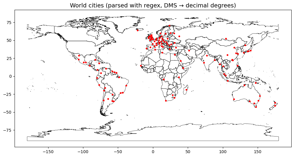

World Cities Map — GeoPandas with Natural Earth basemap

Pipeline: Regex extracts city name, lat/lon (in degrees–minutes format), and country from worldcities.txt → convert DMS to decimal degrees → build Shapely Point geometries → load into a GeoPandas GeoDataFrame → overlay on the Natural Earth basemap to plot the global city distribution.

---

Midterm

Midterm Project — Data Analysis Suite

Three independent Python programs that demonstrate file operations, data analysis, and real-estate query capability.

%%{init: {"theme": "base", "themeVariables": {"fontSize": "18px"}, "flowchart": {"padding": 35}}}%%
flowchart TD
    A["Midterm Project     "] --> B["Alumni Research     "]
    A --> C["File Manipulation     "]
    A --> D["Real Estate Search     "]

    B --> B1["Income & Debt by Major     "]
    C --> C1["Recursive CSV Processing     "]
    D --> D1["Multi-criteria Property Filter     "]

    style A fill:#E3F2FD,color:#1565C0,stroke:#90CAF9,stroke-width:2px
    style B fill:#FFF3E0,color:#E65100,stroke:#FFCC80,stroke-width:2px
    style C fill:#E8F5E9,color:#2E7D32,stroke:#A5D6A7,stroke-width:2px
    style D fill:#F3E5F5,color:#6A1B9A,stroke:#CE93D8,stroke-width:2px
    style B1 fill:#F5F5F5,color:#424242,stroke:#BDBDBD,stroke-width:2px
    style C1 fill:#F5F5F5,color:#424242,stroke:#BDBDBD,stroke-width:2px
    style D1 fill:#F5F5F5,color:#424242,stroke:#BDBDBD,stroke-width:2px

1. Alumni Research

Analyze alumni income and student debt: average age and gender breakdown by major, income ranking, and a loan-payoff calculator (5% of annual income as the monthly payment).

# Loan payoff calculator: 5% annual income as monthly payment
def loan_payoff(debt, annual_income, interest_rate=0.05):
    monthly_payment = annual_income * 0.05 / 12
    balance, months = debt, 0
    while balance > 0:
        balance *= (1 + interest_rate / 12)
        balance -= monthly_payment
        months += 1
    return months // 12, months % 12

2. File Manipulation

Recursively walk a directory tree, detect CSV files, and pretty-print them in tab-separated format.

import os
def process_directory(path):
    if os.path.isfile(path) and path.endswith('.csv'):
        pretty_print_csv(path)
    elif os.path.isdir(path):
        for root, dirs, files in os.walk(path):
            for f in files:
                if f.endswith('.csv'):
                    pretty_print_csv(os.path.join(root, f))

3. Real Estate Search

Multi-criteria property filter: state code, minimum living area, market-value range, and target school district.

Midterm summary: Three programs that exercise (1) pandas data analysis and joining (merge on ID), (2) recursive file processing with os.walk(), and (3) multi-criterion logical filtering. Together they cover data science, system operations, and practical applications.

---

Final Project

SVD Image Compression Application

Task: Build an interactive desktop application for image compression using Singular Value Decomposition (SVD), with real-time preview and quality metrics.

Method: PyQt6 GUI + NumPy SVD + PIL image processing

Mathematical Foundation: Eckart–Young Theorem — A_k = sum(sigma_i · u_i · v_iᵀ) for i = 1 … k

Application Architecture

%%{init: {"theme": "base", "themeVariables": {"fontSize": "18px"}, "flowchart": {"padding": 35}}}%%
flowchart TD
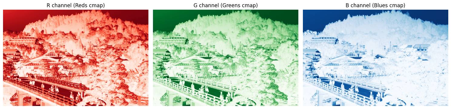
    A["Image Input (drag & drop)     "] --> B["RGB Channel Split     "]
    B --> C["np.linalg.svd per channel     "]
    C --> D["Low-rank Approximation A_k     "]
    D --> E["Reconstruct RGB     "]
    E --> F["PSNR + File Size     "]
    F --> G["Preview & Export     "]

    style A fill:#E3F2FD,color:#1565C0,stroke:#90CAF9,stroke-width:2px
    style B fill:#E3F2FD,color:#1565C0,stroke:#90CAF9,stroke-width:2px
    style C fill:#FFF3E0,color:#E65100,stroke:#FFCC80,stroke-width:2px
    style D fill:#FFF3E0,color:#E65100,stroke:#FFCC80,stroke-width:2px
    style E fill:#E8F5E9,color:#2E7D32,stroke:#A5D6A7,stroke-width:2px
    style F fill:#F3E5F5,color:#6A1B9A,stroke:#CE93D8,stroke-width:2px
    style G fill:#E8F5E9,color:#2E7D32,stroke:#A5D6A7,stroke-width:2px

SVD foundations: Any matrix A decomposes as A = U Σ Vᵀ. Taking the top-k singular values to rebuild A_k yields the best rank-k approximation (Eckart–Young theorem). Smaller k means higher compression but lower quality.

Core Algorithm

import numpy as np
from PIL import Image

def perform_svd(image_array):
    """SVD on each RGB channel separately"""
    channels = {}
    for i, name in enumerate(['R', 'G', 'B']):
        U, S, Vt = np.linalg.svd(image_array[:, :, i], full_matrices=False)
        channels[name] = (U, S, Vt)
    return channels

def reconstruct(channels, k):
    """Low-rank approximation with k singular values"""
    reconstructed = np.zeros_like(original)
    for i, name in enumerate(['R', 'G', 'B']):
        U, S, Vt = channels[name]
        reconstructed[:, :, i] = np.clip(
            U[:, :k] @ np.diag(S[:k]) @ Vt[:k, :], 0, 255
        )
    return reconstructed.astype(np.uint8)

def calculate_psnr(original, compressed):
    mse = np.mean((original.astype(float) - compressed.astype(float)) ** 2)
    return 10 * np.log10(255**2 / mse) if mse > 0 else float('inf')

GUI Features

# PyQt6 GUI with dual slider control
class SVDCompressor(QMainWindow):
    def __init__(self):
        # Drag-and-drop image upload
        # Dual slider: compression ratio ↔ target file size (linked)
        # Smart presets:
        #   Social media: 2 MB, ~35 dB PSNR
        #   Email:        5 MB, ~40 dB PSNR
        #   High quality: 80% compression, ~45 dB PSNR
        pass

Application Demo

SVD Compression App — PyQt6 Desktop Application

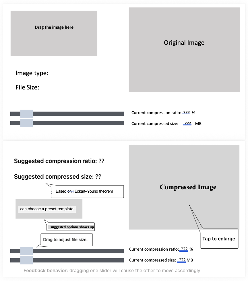
App feature highlights:

• Drag-and-drop upload — drop an image into the window to load it
• Linked dual sliders — compression ratio ↔︎ target file size (moving one auto-updates the other)
• Smart presets — three templates: social media (2 MB), email attachment (5 MB), high-quality archive (PSNR > 40 dB)
• Live preview — side-by-side original vs compressed, with PSNR / file size / compression ratio shown below
• Quality warnings — automatic alert when PSNR drops below 40 dB
• Eckart–Young guarantee — theoretically optimal low-rank approximation

📎 Download: SVD_app.py (source code)

SVD Quality Analysis

RGB Channel Decomposition

SVD Metrics vs k (MSE, PSNR, norm, sigma)

Warning in annotate("label", x = 300, y = 34, label = "k=300: 31.88 dB", :
Ignoring unknown parameters: `label.size`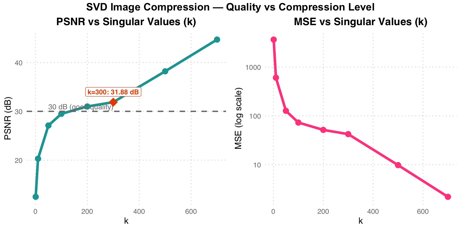

Quality analysis: Left — PSNR rises with k, reaching 31.88 dB at k = 300 (above the 30 dB threshold marked by the grey dashed line) and approaching the original at k = 700 (44.70 dB). Right — MSE drops exponentially, with diminishing returns past k = 300. Practical takeaway: k = 200–400 is the sweet spot between compression and quality.

k	PSNR (dB)	MSE	Compression Ratio
1	12.50	3650	99.9%
50	27.10	127	95.1%
100	29.50	73	90.3%
300	31.88	42.29	70.9%
700	44.70	2.2	32.0%

Eckart–Young verification: Experiments confirm ‖A − A_k‖₂ ≈ σ_{k+1} — the error of the low-rank approximation equals the (k+1)-th singular value. This gives a principled rule for choosing k: stop once σ_{k+1} drops below the desired quality threshold.

---

Course Skills Summary

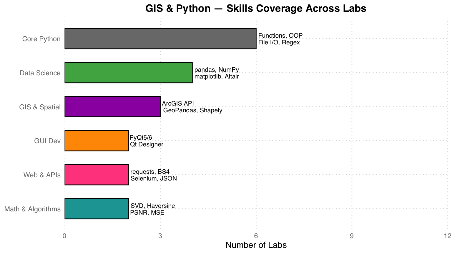
Course wrap-up: From core Python (functions, OOP, file I/O), through data science (pandas, visualization), GIS and spatial analysis (ArcGIS, GeoPandas), GUI development (PyQt5/6), and web scraping (requests, BeautifulSoup), to a final SVD image-compression project that fuses mathematical theory with software-engineering practice.