Big Data Analysis

Big Data Analysis · NCHU Institute of Data Science and Information Computing

Assignments

Reading Assignment — Nystrom Method

Paper: Using the Nystrom Method to Speed Up Kernel Machines Authors: Christopher K. I. Williams & Matthias Seeger (NIPS 2000)

Paper Summary: The main bottleneck of kernel-based methods (such as SVM, Gaussian Process) lies in the computation and matrix inversion of the Gram matrix, with a time complexity of O(n^3). This paper proposes using the Nystrom method to approximate the Gram matrix — sampling only m points from n training data points, computing a small matrix, and then expanding it into a full approximation, reducing the computation from O(n^3) to O(m^2n).

Core Idea

%%{init: {"theme": "base", "themeVariables": {"fontSize": "18px"}, "flowchart": {"padding": 35}}}%%
flowchart LR
    A["Full Gram Matrix K (n×n)     "] --> B["Sample m points     "]
    B --> C["K_mm (m×m)     "]
    B --> D["K_nm (n×m)     "]
    C --> E["Eigen-decompose K_mm     "]
    D --> F["Nyström Approx:\nK ≈ K_nm K_mm⁻¹ K_nm^T     "]

    style A fill:#FCE4EC,color:#C62828,stroke:#F48FB1,stroke-width:2px
    style B fill:#F5F5F5,color:#424242,stroke:#BDBDBD,stroke-width:2px
    style C fill:#E3F2FD,color:#1565C0,stroke:#90CAF9,stroke-width:2px
    style D fill:#E3F2FD,color:#1565C0,stroke:#90CAF9,stroke-width:2px
    style E fill:#FFF3E0,color:#E65100,stroke:#FFCC80,stroke-width:2px
    style F fill:#E8F5E9,color:#2E7D32,stroke:#A5D6A7,stroke-width:2px

Nystrom Workflow: From the full n x n Gram matrix (pink, extremely costly to compute), m samples are randomly selected to form the blue sub-matrices K_mm and K_nm, then reconstructed via eigen-decomposition (orange) into the green approximate matrix. This yields significant speedup when m << n.

Key Formulas

Mercer Expansion (Kernel Expansion):

\[K(x, y) = \sum_{i=1}^{\infty} \lambda_i \phi_i(x) \phi_i(y)\]

Nystrom Approximation:

\[\tilde{K} = K_{nm} K_{mm}^{-1} K_{nm}^T\]

Complexity Reduction:

\[O(n^3) \rightarrow O(m^2 n), \quad m \ll n\]

---

Homework — Nystrom Kernel Ridge Classification

Task: Implement the Nystrom method to accelerate RBF Kernel Ridge Classification on the USPS handwritten digit dataset (binary: digit “4” vs. rest).

Dataset: USPS — 7,291 training + 2,007 test images, 256 features (16x16 pixels)

Method: RBF Kernel (sigma=4) + Ridge Regression (lambda=0.001) + Nystrom Approximation (m = 128, 256, 512)

Pipeline Overview

%%{init: {"theme": "base", "themeVariables": {"fontSize": "18px"}, "flowchart": {"padding": 35}}}%%
flowchart LR
    A["USPS 7291×256     "] --> B["StandardScaler     "] --> C["RBF Kernel σ=4     "]
    C --> D["Full: K (7291×7291)     "]
    C --> E["Nyström: K_mm + K_nm     "]
    D --> F["Ridge Solve     "]
    E --> F
    F --> G["Predict ±1     "]

    style A fill:#E3F2FD,color:#1565C0,stroke:#90CAF9,stroke-width:2px
    style B fill:#F5F5F5,color:#424242,stroke:#BDBDBD,stroke-width:2px
    style C fill:#FFF3E0,color:#E65100,stroke:#FFCC80,stroke-width:2px
    style D fill:#FCE4EC,color:#C62828,stroke:#F48FB1,stroke-width:2px
    style E fill:#E8F5E9,color:#2E7D32,stroke:#A5D6A7,stroke-width:2px
    style F fill:#E3F2FD,color:#1565C0,stroke:#90CAF9,stroke-width:2px
    style G fill:#E8F5E9,color:#2E7D32,stroke:#A5D6A7,stroke-width:2px

Pipeline Description: USPS data is first standardized, then split into two paths: pink Full Kernel computes the complete 7291x7291 Gram matrix, while green Nystrom only computes the subset matrices K_mm + K_nm. Both solve the coefficient vector alpha via Ridge Regression, and ultimately predict +/-1.

Implementation

# RBF Kernel function
def rbf_kernel(X1, X2, sigma=4.0):
    sq_dists = (np.sum(X1**2, axis=1)[:, None]
                + np.sum(X2**2, axis=1)[None, :]
                - 2 * X1 @ X2.T)
    return np.exp(-sq_dists / (2 * sigma**2))

# Kernel Ridge: solve (K + λI) α = y
def kernel_ridge_train(K, y, lam=1e-3):
    n = K.shape[0]
    return np.linalg.solve(K + lam * np.eye(n), y)

# Nyström approximation
def nystrom_approximation(X_train, m, sigma=4.0):
    indices = np.random.choice(n, m, replace=False)
    X_sub = X_train[indices]
    K_mm = rbf_kernel(X_sub, X_sub, sigma)
    K_nm = rbf_kernel(X_train, X_sub, sigma)
    K_mm_inv = np.linalg.inv(K_mm + 1e-8 * np.eye(m))
    K_approx = K_nm @ K_mm_inv @ K_nm.T
    return K_approx, indices, K_nm, K_mm_inv

Results

Method	Errors	Accuracy	Train Time (s)
Full Kernel	9	99.55%	7.52
Nystrom m=128	10	99.50%	0.38
Nystrom m=256	10	99.50%	0.63
Nystrom m=512	9	99.55%	1.83

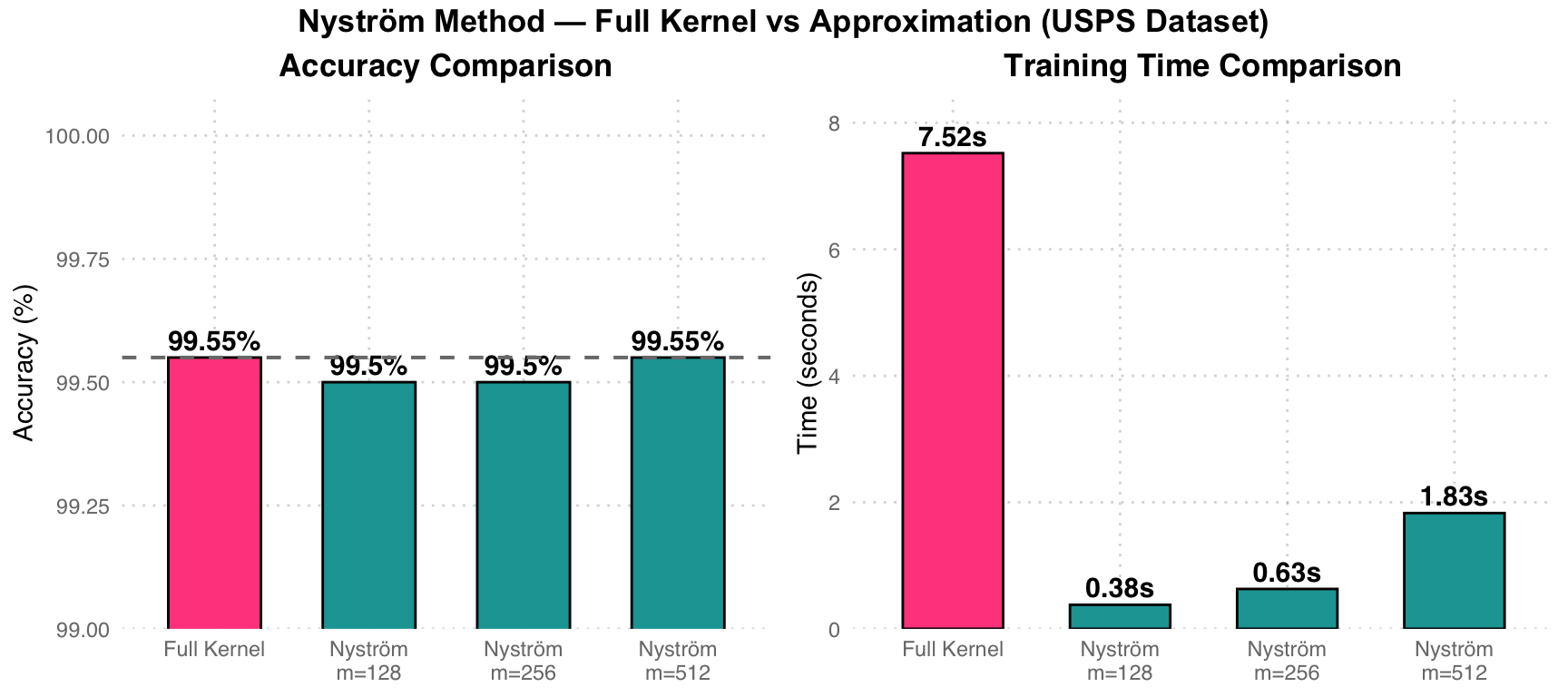
Performance Analysis: Pink Full Kernel takes 7.52 seconds to compute the complete 7291x7291 Gram matrix. Teal Nystrom m=128 takes only 0.38 seconds (approximately 20x speedup), with accuracy nearly unchanged (99.50% vs 99.55%). At m=512, precision fully matches Full Kernel, while training time is still reduced by 75%.

Gram Matrix Visualization

Full Kernel vs Nystrom Approximation (first 100 samples)

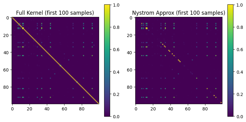
Matrix Comparison: The left figure shows the full Gram matrix (first 100 samples), and the right figure shows the Nystrom approximation result. The two are highly similar in structure, validating that the Nystrom method significantly reduces computation while preserving the kernel structure.

---

Final Project

Smoothed & Distributed SVM

Task: Implement and compare three SVM variants: (1) standard LinearSVC, (2) Smoothed SVM using log-sum-exp approximation of hinge loss, and (3) Distributed Smoothed SVM with communication-efficient gradient aggregation.

Dataset: a9a (Adult Income) — 32,561 training + 16,281 test samples, 123 features

Method: LinearSVC baseline -> Smoothed Hinge Loss (beta=5) + L-BFGS-B -> Distributed SGD (K=5 workers)

Three SVM Variants

%%{init: {"theme": "base", "themeVariables": {"fontSize": "18px"}, "flowchart": {"padding": 35}}}%%
flowchart TD
    DATA["a9a Dataset 32K×123     "] --> S1["LinearSVC (sklearn)     "]
    DATA --> S2["Smoothed SVM (L-BFGS-B)     "]
    DATA --> S3["Distributed Smooth SVM     "]

    S1 --> R1["Baseline Accuracy     "]
    S2 --> R2["Single-node Accuracy     "]
    S3 --> |"K=5 workers"| R3["Distributed Accuracy     "]

    S3 --> W1["Worker 1     "]
    S3 --> W2["Worker 2     "]
    S3 --> W3["...     "]
    S3 --> W4["Worker 5     "]

    style DATA fill:#E3F2FD,color:#1565C0,stroke:#90CAF9,stroke-width:2px
    style S1   fill:#F5F5F5,color:#424242,stroke:#BDBDBD,stroke-width:2px
    style S2   fill:#FFF3E0,color:#E65100,stroke:#FFCC80,stroke-width:2px
    style S3   fill:#E8F5E9,color:#2E7D32,stroke:#A5D6A7,stroke-width:2px
    style R1   fill:#F5F5F5,color:#424242,stroke:#BDBDBD
    style R2   fill:#FFF3E0,color:#E65100,stroke:#FFCC80
    style R3   fill:#E8F5E9,color:#2E7D32,stroke:#A5D6A7
    style W1   fill:#E8F5E9,color:#2E7D32,stroke:#A5D6A7
    style W2   fill:#E8F5E9,color:#2E7D32,stroke:#A5D6A7
    style W3   fill:#E8F5E9,color:#2E7D32,stroke:#A5D6A7
    style W4   fill:#E8F5E9,color:#2E7D32,stroke:#A5D6A7

Architecture Overview: Grey = sklearn LinearSVC baseline, orange = single-node Smoothed SVM (L-BFGS-B optimization), green = distributed version (K=5 workers, each worker computes local gradients per round then aggregates).

Smoothed Hinge Loss

Standard hinge loss is non-differentiable at u=1. The smoothed version uses log-sum-exp to create a differentiable approximation:

\[\ell_\beta(u) = \frac{1}{\beta} \log\left(1 + e^{\beta(1-u)}\right)\]

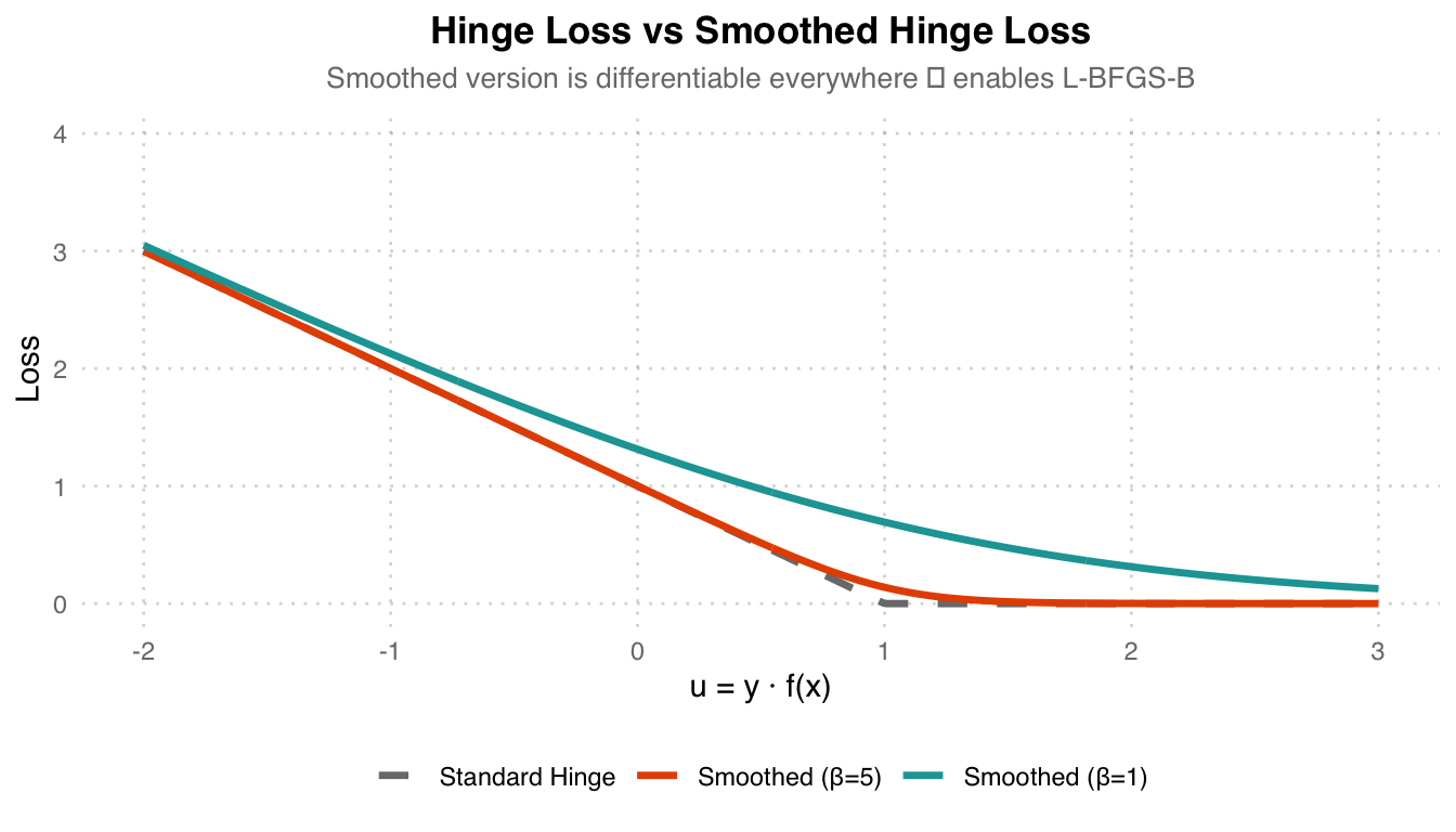
Loss Comparison: Grey dashed line Standard Hinge Loss is non-differentiable at u=1. Orange Smoothed (beta=5) provides the closest approximation to the original hinge while being differentiable everywhere. Teal (beta=1) is smoother but deviates more from the original hinge. The larger the beta, the closer it is to the original shape.

Distributed Gradient Aggregation

# Distributed Smoothed SVM — Communication-efficient gradient
K = 5  # number of workers
B = 5  # communication rounds
beta = np.zeros(X_train.shape[1])

for b in range(B):
    # Pilot gradient (computed on worker 0)
    grad_pilot = compute_gradient(beta, X_pilot, y_pilot, lambda_, beta_smooth)

    # Each worker computes local gradient correction
    grad_total = np.zeros_like(beta)
    for X_k, y_k in zip(split_X, split_y):
        grad_k = compute_gradient(beta, X_k, y_k, lambda_, beta_smooth)
        grad_total += (grad_k - grad_pilot) * (len(X_k) / len(X_train))

    # Aggregate: surrogate gradient = pilot + corrections
    beta -= 0.1 * (grad_pilot + grad_total)

Distributed Strategy: Data is split into K=5 partitions. Each round, only one pilot worker computes the full gradient, while the remaining workers compute “gradient differences from the pilot” (correction terms), which are then aggregated. Compared to having every worker transmit full gradients, this method significantly reduces communication overhead.

Results

Model	Test Accuracy	Training Time
LinearSVC (sklearn baseline)	84.93%	1.52s
Smoothed SVM (single-node, L-BFGS-B)	84.88%	0.78s
Distributed Smoothed SVM (K=5, B=5)	83.79%	0.01s

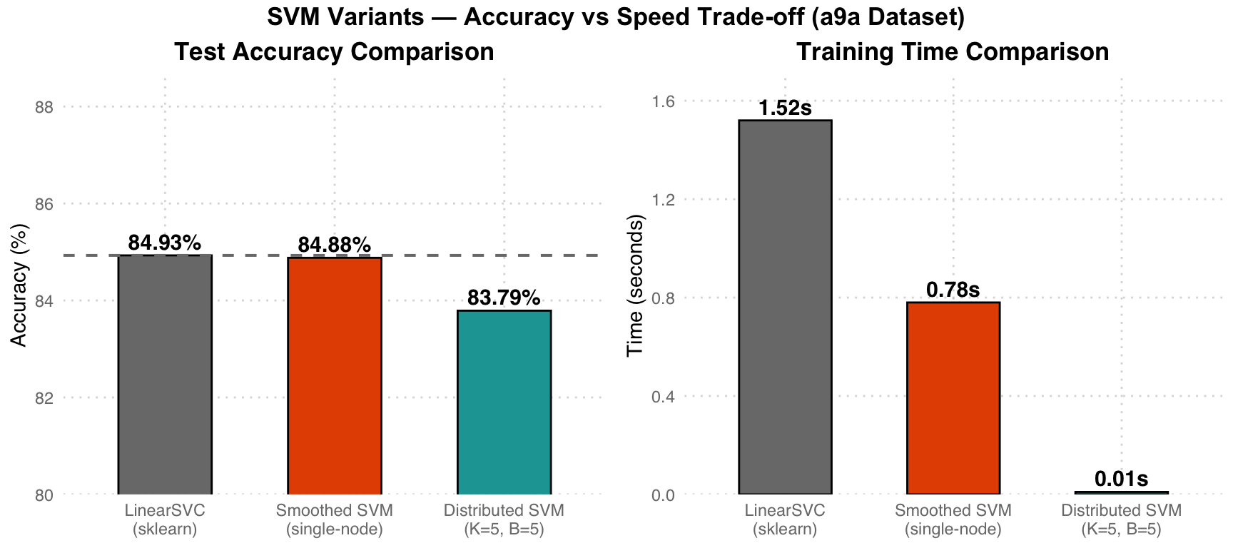
Trade-off Analysis: Grey LinearSVC serves as the baseline (84.93%). Orange Smoothed SVM achieves nearly identical accuracy (84.88%), but is faster due to more efficient L-BFGS-B optimization (0.78s vs 1.52s). Teal Distributed version sacrifices ~1.1% accuracy in exchange for 150x speedup (0.01s), demonstrating the potential of distributed computing for large-scale data.

Ablation Study — Beta Sensitivity

Beta (smoothness)	Test Accuracy
1	83.69%
2	83.79%
5	83.79%
10	83.73%
20	81.21%

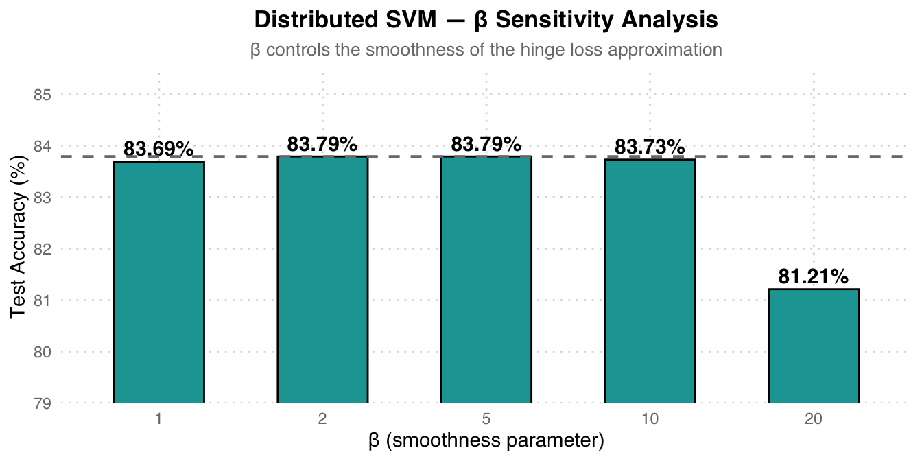
Beta Selection Recommendation: Beta=2 and beta=5 perform best with identical results (83.79%). A beta that is too large (=20) actually causes accuracy to drop to 81.21%, because over-approximating the non-differentiable original hinge loss leads to unstable gradient estimates. Beta=5 is the optimal balance point.