Tzu-Yuan Chen

Assignments

Assignment 1

Question 1

Name and describe three applications you have used that employed a database system to store and access persistent data. (e.g. airlines, online trade, banking, university system)

For the first question, one example that comes to mind is video games. In video games, a player’s level and experience points, as well as the items and equipment they have obtained, are recorded, so the player can still access them the next time they log in. Another example is online shopping. For instance, Amazon records information such as the price of each product, the catalog it belongs to, whether it is eligible for free shipping, and whether it is in stock. A third example is a streaming platform, such as Netflix, which records a user’s region and subscription level. All of this data is stored persistently and can be accessed at a later time.

Question 2

Propose three applications in domain projects (e.g. criminology, economics, brain science, etc.) Be sure you include: i. Purpose ii. Functions iii. Simple interface design

Wardrobe Management Database

i. Purpose

The main purpose of this wardrobe management database is to minimize the time spent choosing outfits before going out.

For many people, the difficulty in daily outfit selection is not a lack of clothing, but the need to simultaneously consider colors, styles, occasions, and overall coordination, which leads to a high decision-making cost.

Therefore, I model the wardrobe as a relational database, which not only records individual clothing items but also describes the relationships between items, allowing outfit selection to be handled in a systematic way.

By structuring clothing data, this system aims to transform “rethinking what to wear every day” into “quickly selecting optimal combinations from a database.”

ii. Functions

In this system, each clothing item is treated as a data entity and described using a set of attributes, such as:

category (T-shirts, jeans, outerwear, shoes),
color (including the proportion of each color),
style (clean-fit, formal, vintage, sports, etc.),
material (denim, linen, cotton).

These attributes are normalized into multiple tables, and many-to-many relationships are used to represent that a single item can belong to multiple styles or be suitable for different occasions.

The core function of this database is not only to store items, but to describe the compatibility between items.

The system uses compatibility rules to define:

Visual aesthetic constraints, such as avoiding more than three colors in a single outfit and limiting the number of style tags to maintain overall consistency
Climate adaptability, where combinations are evaluated based on insulation-related variables to ensure balanced warmth between upper and lower body layers, and higher overall insulation is preferred as the temperature decreases

When a user selects a specific item (for example, a pink T-shirt), the system can immediately recommend other highly compatible items (such as light blue jeans and white sneakers) based on database relationships and rules, and rank these combinations by compatibility score to help the user make decisions more efficiently.

In addition, as data accumulates, the system can analyze the overall structure of the wardrobe, such as:

Whether certain styles or clothing categories are lacking
Whether colors or item types are overly concentrated
Whether newly purchased items overlap in function with existing ones
Which older items have not been used for a long time and could be considered for removal

This allows the wardrobe to function not just as an item list, but as a system that can be queried, analyzed, and optimized, and that can be extended to daily life applications such as outfit recommendations and purchase decision support.

This problem is particularly well suited for a relational database, because outfit selection inherently involves structured data and many-to-many relationships (such as items, styles, and compatibility rules), which can be efficiently combined and analyzed through relational queries.

iii. Simple interface design

When users enter the system, the home page displays a table view of all items in the wardrobe, including basic information such as category, color, style, material, and seasonality. The interface supports multi-select functionality.

Users can select one or more items they plan to wear and submit their selection to generate outfit results.

Based on the selected items and the compatibility rules stored in the database, the system generates multiple outfit candidates.

The outfit results page provides different sorting options, such as sorting by comfort score, aesthetic score, or climate fit score.

Each outfit displays its corresponding numerical scores, allowing users to quickly compare options and select the most suitable combination without repeatedly trying on clothes or overthinking the decision.

The interface supports fast decision-making: select items → generate outfits → sort by scores → pick the best match.

3D Printing Farm Order & Scheduling Database

i. Purpose

The purpose of this 3D printing farm database is to systematize the entire workflow—from customer order intake to automated estimation, machine scheduling, and progress tracking—so the farm can operate efficiently as order volume grows. The goals are to shorten turnaround time, reduce human scheduling errors, improve machine utilization, and maximize profitability.

In practice, 3D printing orders vary widely (model size, material, resolution, multi-color requirements, and post-processing such as painting). If pricing and scheduling rely on manual judgment, it is easy to underestimate time/cost, assign the wrong machine, or create bottlenecks in the order queue. Therefore, this system uses a relational database to store orders, machine capabilities, material usage, and scheduling states in a structured way, enabling fast and consistent decisions through rules and queries.

ii. Functions

Order intake & requirement tagging (Order Intake & Requirement Tagging)

When a customer submits an order, the system stores it as an order record with structured attributes, such as:

Model size and volume (bounding box / volume)
Printing type (FDM / SLA)
Resolution settings (layer height / resolution)
Multi-color requirement (multi-color)
Material type (material type)
Post-processing needs (post-processing, e.g., painting/sanding)
Other customization requests (stored as tags)

These fields can be normalized into multiple tables, with many-to-many relationships used to represent that a single order can have multiple requirement tags.

Per-machine estimation (Per-Machine Estimation)

The key is not only to calculate an overall price for the order, but to estimate how the same order would perform on different machines, since time, cost, and completion time may vary by machine. This supports better machine assignment and scheduling decisions.

For each candidate machine, the system applies pricing rules or an estimation model to perform per-machine estimation, including:

Estimated print time (estimated print time)
Estimated material usage (estimated material usage)
Machine-specific estimated cost & quote (machine-specific estimated cost & quote)
Estimated completion time (estimated completion time, considering current workload)

The system stores these “order × machine” estimates for querying and ranking using different objective functions, such as lowest cost, earliest completion, or the most stable option within a deadline.

Order queue & status tracking (Order Queue & Status Tracking)

All orders are automatically added to an order queue (order list), and each order maintains a clear status, such as:

pending
queued
printing
post-processing
completed
failed

Managers can query:

What is currently in the queue and its priority
Which orders are printing vs. waiting for machines
Which failed orders require reprinting or manual intervention

Machine capability modeling & assignment recommendations (Machine Capability & Assignment)

The database stores each machine’s capabilities and constraints, such as: - Machine type: multi-color / single-color / SLA / FDM - Maximum build volume (max build volume) - Supported materials (supported materials) - Speed/quality profile (speed/quality profile) - Current workload and availability (workload & availability)

When a new order arrives, the system first performs constraint filtering (e.g., size, material, multi-color requirements) to identify feasible machines, then uses per-machine estimation to generate recommended assignments, for example:

Earliest completion time (earliest completion time)
Lowest estimated cost (lowest estimated cost)
Balanced option (deadline + stability)

This turns scheduling into a decision-support process rather than manual guesswork.

iii. Simple interface design

On the customer side, the system provides a customer order page where users can upload a 3D model or specify printing requirements such as size, material, resolution, multi-color options, and post-processing needs. Based on this information, the system automatically returns an estimated price and an estimated delivery time.

On the admin side, the system offers an order dashboard that displays the current order queue and order statuses. Administrators can sort or filter orders by deadline, priority, or processing status to manage workflow more efficiently.

The system also includes a machine dashboard that lists all available machines along with their machine type, maximum build volume, supported materials, current workload, and estimated availability. This allows operators to quickly understand machine capacity and constraints.

When an order is selected, the scheduling view presents a list of candidate machines that can fulfill the order. For each candidate machine, the system displays the estimated print time, estimated material usage, machine-specific cost and quote, and estimated completion time. The interface supports one-click sorting options, such as fastest, cheapest, or most stable, to assist administrators in making assignment decisions.

The interface supports efficient operations: submit order → per-machine estimation → queue order → recommend machines → schedule & track progress.

Wardrobe Management Database

i. Purpose

The purpose of this system is to manage the core information of a farm—such as fields, crop types, growth stages, and irrigation equipment—using a relational database.

At the same time, the system retrieves and stores weather data through APIs provided by weather forecast services, and combines this information with a set of irrigation rules to automatically generate a daily irrigation schedule.

The goal is to reduce manual decision-making costs while improving water-use efficiency and consistency in crop management.

ii. Functions

In this system, the database is not used only for data storage. Its core function is to integrate internal farm information with external weather data and automatically generate irrigation decisions based on predefined rules.

Core Data Management

The system uses a relational schema to manage the main entities of the farm, including:

Field: field ID, location, area, and the crop currently planted
Crop: crop type and its basic water requirements
Growth Stage: stages such as germination, growth, flowering, and fruiting, each with different water needs
Irrigation Equipment: equipment type (e.g., drip irrigation, sprinkler), flow rate or efficiency factor, and availability status

These entities are connected through relationships. For example, each field is associated with a specific crop and a current growth stage, and can be assigned available irrigation equipment.

Weather Data Integration

The system retrieves weather information through external weather forecast APIs, such as:

Predicted rainfall amount
Probability of precipitation
Temperature range

This weather data is stored in the database and used as an important input for daily irrigation decisions, without requiring manual input from users.

Irrigation Rules and Schedule Generation

The system maintains a set of irrigation rules that describe irrigation requirements under different conditions, such as:

Crop type × growth stage → recommended baseline irrigation amount
If predicted rainfall exceeds a certain threshold → automatically reduce or cancel irrigation for the day
Differences in irrigation equipment efficiency → adjust actual irrigation duration

When the daily scheduling process runs, the system combines:

The crop type and growth stage of each field
The weather forecast for the day
The availability and efficiency of irrigation equipment

Based on this information, the system automatically generates a daily irrigation schedule, indicating whether each field requires irrigation and the recommended water amount or irrigation time.

iii. Simple interface design

When users enter the system, the home page displays a table view of all fields on the farm, including the current crop type, growth stage, and the system’s irrigation recommendation for the day.

Users can generate the daily irrigation schedule with a single action. Based on field information, weather forecasts, and irrigation rules, the system lists which fields require irrigation and provides recommended water amounts or irrigation durations.

The schedule is presented in a simple list format, allowing users to quickly review and execute irrigation tasks. After completion, users can mark irrigation status for record-keeping and future reference.

Question 5

What are the things current database system cannot do?

Current database systems are not capable of understanding the semantics behind data. As a result, in more complex applications, they often rely on manually defined rules or continuously adjusted weights to produce reasonable outputs. In addition, databases are limited in handling cross-context decision-making, where multiple competing objectives must be balanced simultaneously.

For example, in a wardrobe management database, the system can evaluate outfits based on structured criteria such as color combinations, style tags, material properties, and weather conditions. It can assign scores for factors like aesthetic quality, comfort, and climate suitability, and generate multiple candidate outfits that satisfy predefined rules. However, the database cannot determine which outfit represents the optimal balance among being visually appealing, comfortable, and suitable for the weather.

This limitation arises because preferences such as “looking good” or “feeling comfortable” are inherently subjective and context-dependent, and there is no single optimal solution that applies to all users or situations. Therefore, the role of the database is not to make the final decision, but to support decision-making by filtering infeasible options, structuring relevant information, and presenting comparable alternatives with transparent evaluation metrics.

Ultimately, the final choice must be made by the user, who can decide whether to prioritize comfort, aesthetics, or climate suitability in a given context. This highlights a fundamental limitation of current database systems: they are effective at decision support, but they cannot replace human judgment in complex, value-driven decisions.

Question 6

Describe at least three tables that might be used to store information in a social-network/social media system such as Twitter or Reddit.

A social-network or social media system such as Twitter or Reddit may be supported by at least the following three core tables:

1. User Table

The user table stores basic information about users, such as: - user_id - username - account creation time - profile metadata (e.g., bio or status)

This table represents the identities of users and serves as a reference for other tables in the system.

2. Post Table

The post table stores content created by users, such as:

post_id
author_id (foreign key referencing the User table)
content
timestamp

Each post is associated with a specific user, forming a one-to-many relationship between users and posts.

3. Comment Table

The comment table stores replies to posts (or other comments), such as:

comment_id
post_id (foreign key referencing the Post table)
author_id
content
timestamp

This table supports threaded discussions and allows multiple users to participate in conversations under the same post.

These tables are separated to support relational queries, maintain data consistency, and enable efficient retrieval of users, posts, and discussion threads.

Assignment 2

Question 1

What are the differences between relation schema, relation, and instance? Give an example using the university database to illustrate.

Relation Schema = The logical structure of a relation: a list of attribute names and their domains. It does not change over time.
Example: instructor(ID, name, dept_name, salary)
Relation = Informally used to refer to both the schema and instance together.
Example: “The department relation” can refer to either the schema department(dept_name, building, budget) or the actual data it currently holds.
Instance = A snapshot of the actual data in a relation at a given point in time. It changes as tuples are inserted, updated, or deleted.
Example: The department relation instance in Figure 2.5 contains 7 tuples. If the university adds a “Data Science” department, the instance grows to 8 tuples, but the schema remains department(dept_name, building, budget).

Question 2 & 3

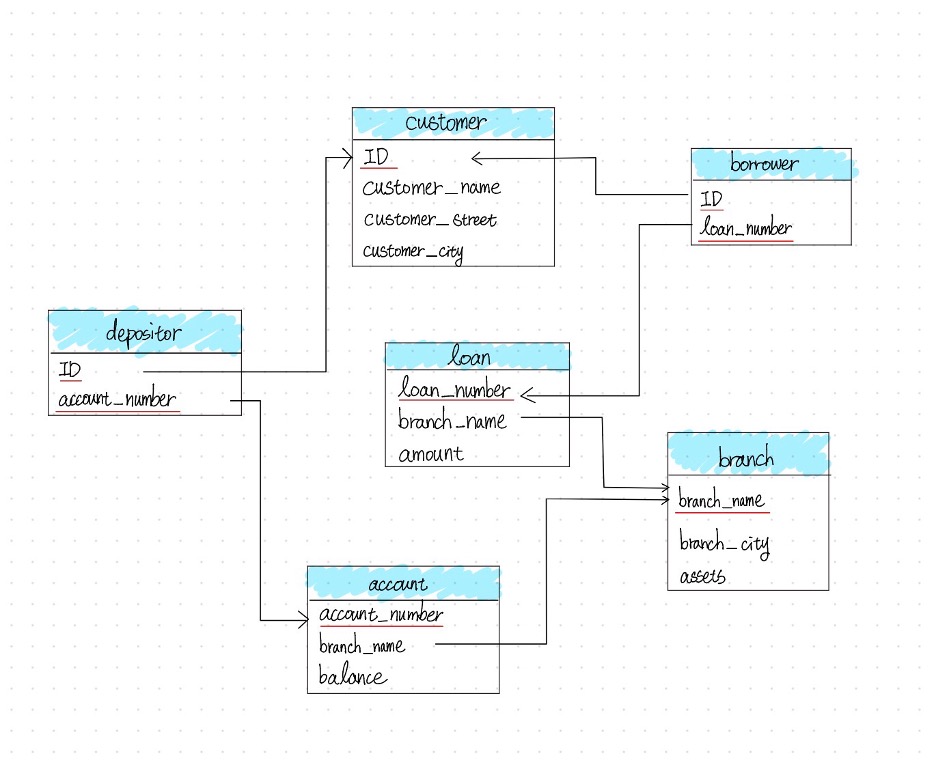
Draw a schema diagram for the following bank database. Identify primary keys (underlined) and foreign keys.

The bank database consists of the following relations:

branch(branch_name, branch_city, assets)
customer(ID, customer_name, customer_street, customer_city)
loan(loan_number, branch_name, amount)
borrower(ID, loan_number)
account(account_number, branch_name, balance)
depositor(ID, account_number)

Question 4

Describe two ways artificial intelligence or LLM can assist in managing or querying a database. In your answer, briefly explain how each method improves efficiency or accuracy compared to traditional (non-AI) approaches. (3–5 sentences)

Natural Language to SQL (Querying): LLMs can translate plain language questions directly into executable SQL queries, lowering the barrier for non-technical users and reducing syntax errors compared to writing SQL manually.
AI-Driven Database Tuning (Managing): LLMs can automatically analyze slow queries and recommend index optimizations, replacing the traditionally time-consuming process of a DBA manually examining query logs and execution plans.

Overall, both approaches reduce the need for specialized expertise and allow faster, more accurate database operations compared to traditional manual methods.

Assignment 3

Question 1

Open the Online SQL interpreter and load the university database.

Question 2

Write SQL codes to get a list of: i. Student IDs, ii. Instructors, iii. Departments

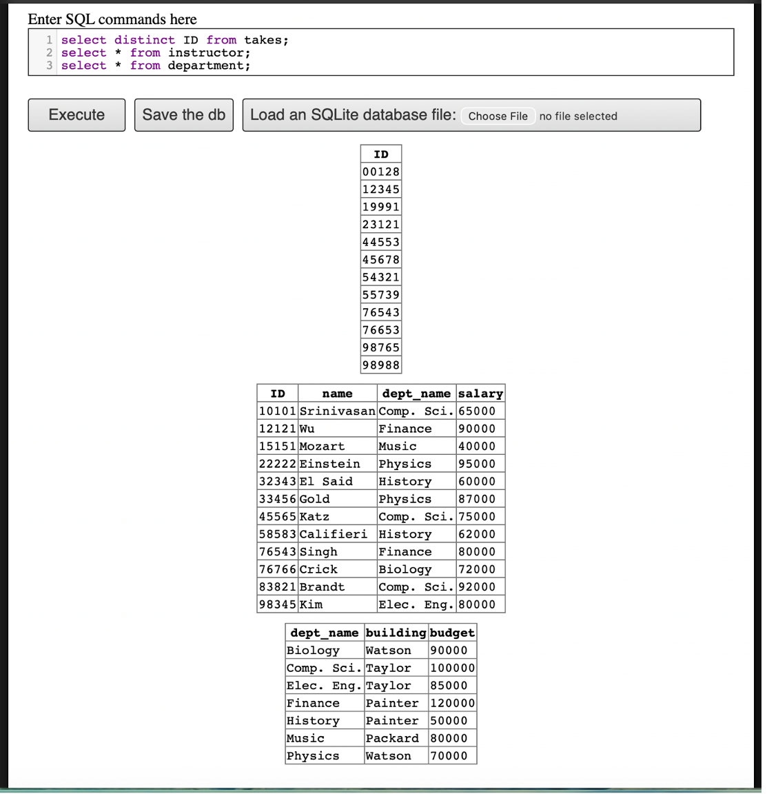
Q2 — Student IDs (from `takes`), Instructors, and Departments

Question 3

Write SQL codes to do the following queries:

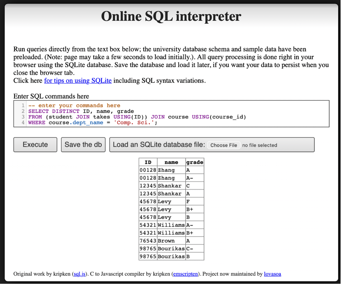
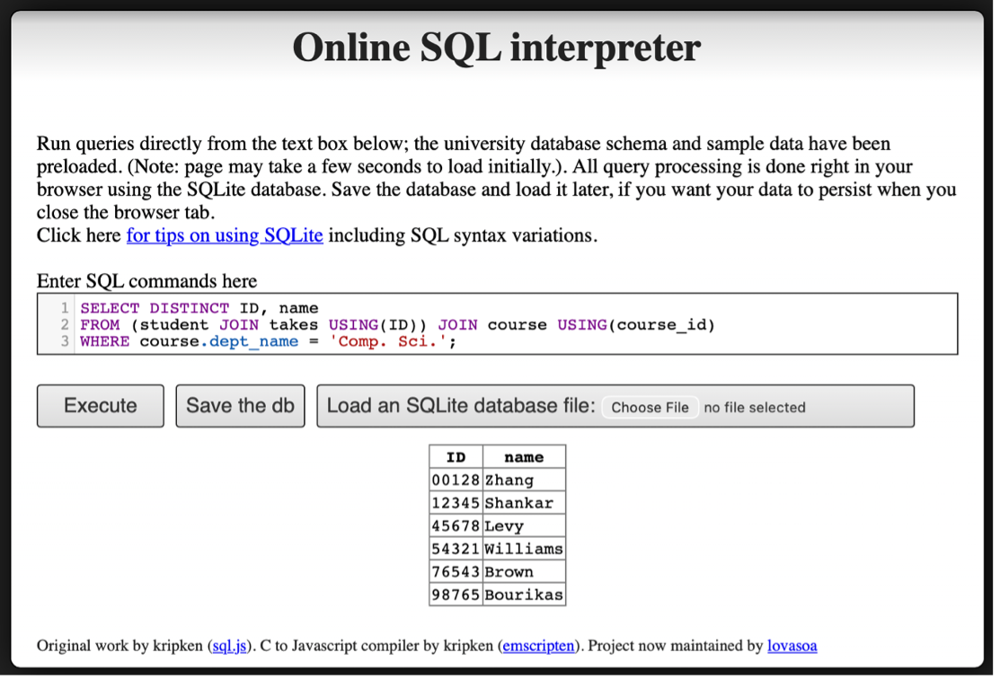
i. Find the ID and name of each student who has taken at least one Comp. Sci. course; make sure there are no duplicate names in the result.

Q3i — Students who took at least one Comp. Sci. course

ii. Add grades to the list

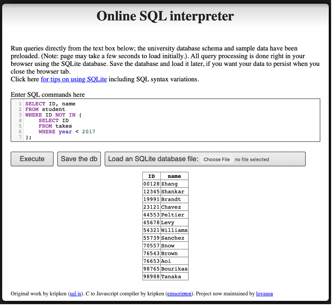
iii. Find the ID and name of each student who has not taken any course offered before 2017.

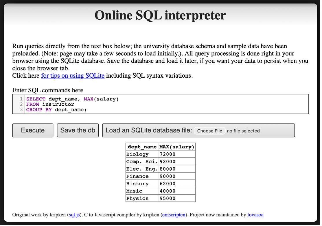
Q3iii — Students who have not taken any course before 2017

iv. For each department, find the maximum salary of instructors in that department.

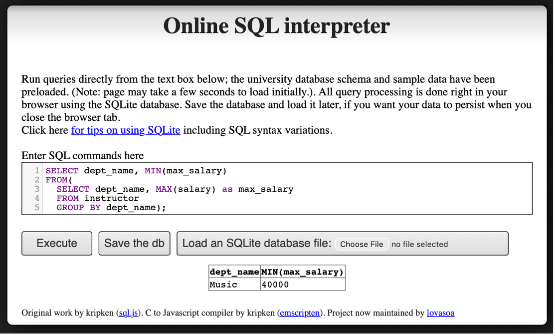
Q3iv — Maximum instructor salary per department

v. Find the lowest, across all departments, of the per-department maximum salary computed by the preceding query.

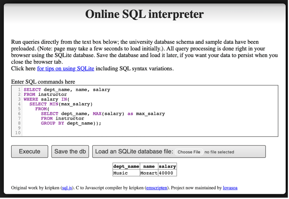
Q3v — Lowest of the per-department maximum salaries

vi. Add names to the list

Q3vi — Add instructor names to the result

Question 4

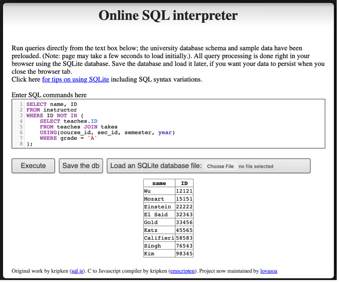
Find instructor (with name and ID) who has never given an A grade in any course she or he has taught. (Instructors who have never taught a course trivially satisfy this condition.)

Q4 — Instructors who have never given an A grade

Assignment 4

Question 1

Explain the difference between a weak entity set and a strong entity set. Use an example other than the one in Chapter 6 to illustrate. (Consult Ch. 6, 6.5.3)

A strong entity set is an entity set that has a primary key of its own and can exist independently. For example, an Order entity with order_id as its primary key can uniquely identify each order without relying on any other entity.

A weak entity set is an entity set that does not have a sufficient set of attributes to form a primary key on its own. Instead, it depends on a related strong entity set (called the identifying entity set) for its identification. A weak entity set uses a discriminator (also called a partial key) that, when combined with the primary key of the identifying entity, uniquely identifies each entity in the weak set.

Example: Order and Order Item

Consider an e-commerce system:

Order is a strong entity set with primary key order_id.
Order_Item is a weak entity set with discriminator item_number.

An Order_Item cannot be uniquely identified by item_number alone, because “item number 3” is meaningless without knowing which order it belongs to. The full identification requires: order_id (from the identifying entity Order) + item_number (the discriminator).

The relationship between Order and Order_Item is an identifying relationship, which means the existence of an Order_Item depends entirely on the existence of its associated Order.

E-R Diagram Notation:

Weak entity set: drawn with a double-border rectangle
Discriminator: marked with a dashed underline
Identifying relationship: drawn with a double-border diamond
The connection from the weak entity to the identifying relationship uses a double line (total participation), because every weak entity must be associated with an identifying entity

Question 2

Design an E-R diagram for keeping track of the scoring statistics of your favorite sports team. You should store the matches played, the scores in each match, the players in each match, and individual player scoring statistics for each match. Summary statistics should be modeled as derived attributes with an explanation as to how they are computed.

a) E-R diagram for a single team (Liverpool FC)

The diagram models two entities: match and player, connected by a many-to-many relationship played. The relationship attributes points_scored, minutes_played, and starter_flag record individual player statistics for each match. Derived attributes on player include total_points() and avg_points_per_match().

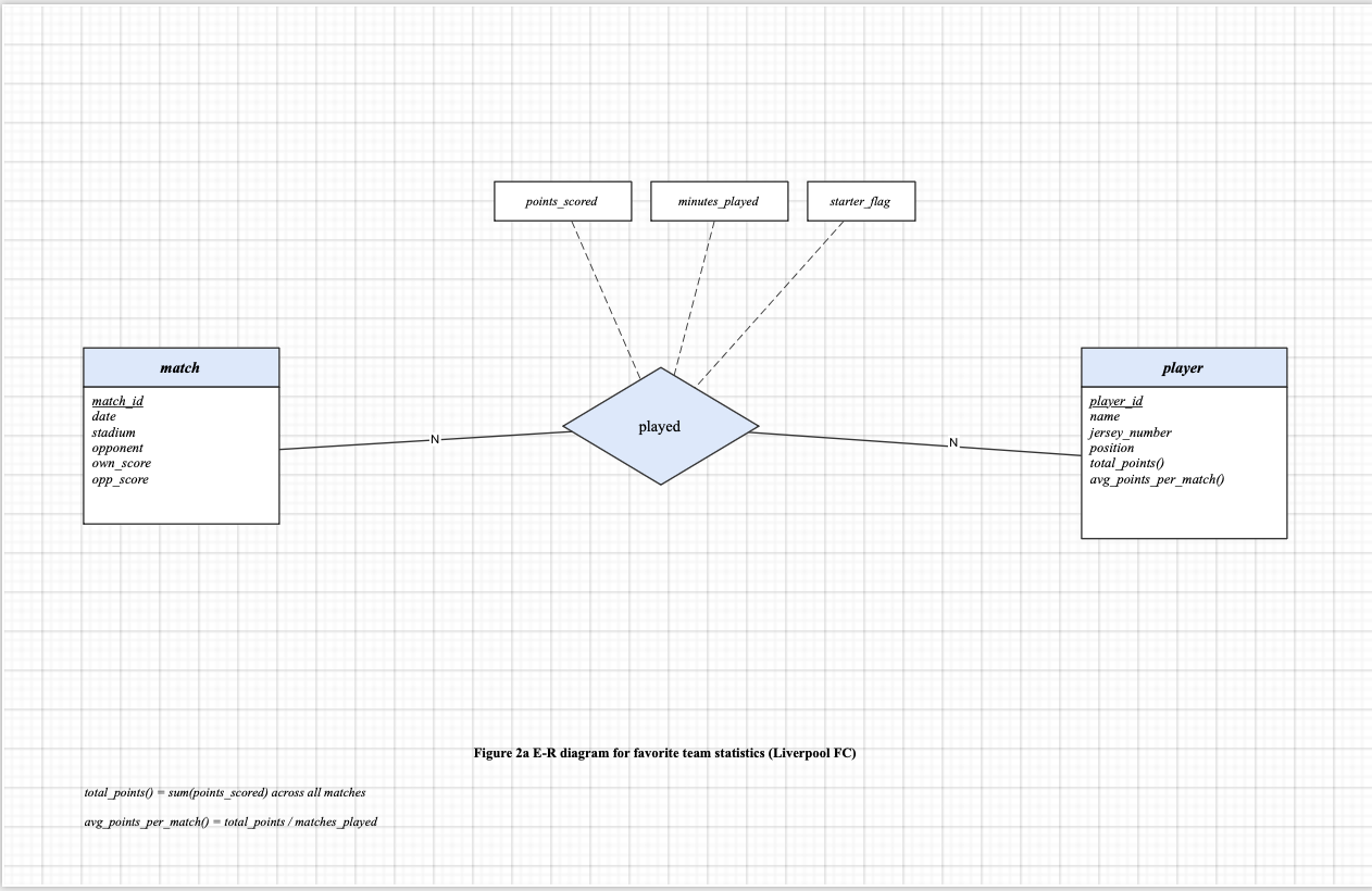
Figure 2a — E-R diagram for favorite team statistics (Liverpool FC)

Derived attribute definitions:

total_points() = sum(points_scored) across all matches
avg_points_per_match() = total_points / matches_played

b) Expanded to all teams in the league

A team entity is added with attributes team_id, team_name, city, and derived attribute win_count(). Two new relationships connect team to match: home_team and away_team. A belongs_to relationship connects player to team (N:1). The match entity is updated with home_team_score, away_team_score, and derived attribute winner().

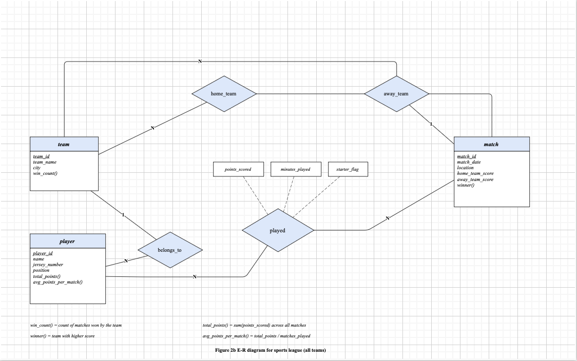
Figure 2b — E-R diagram for sports league (all teams)

Additional derived attribute definitions:

win_count() = count of matches won by the team
winner() = team with higher score

Question 3

3a

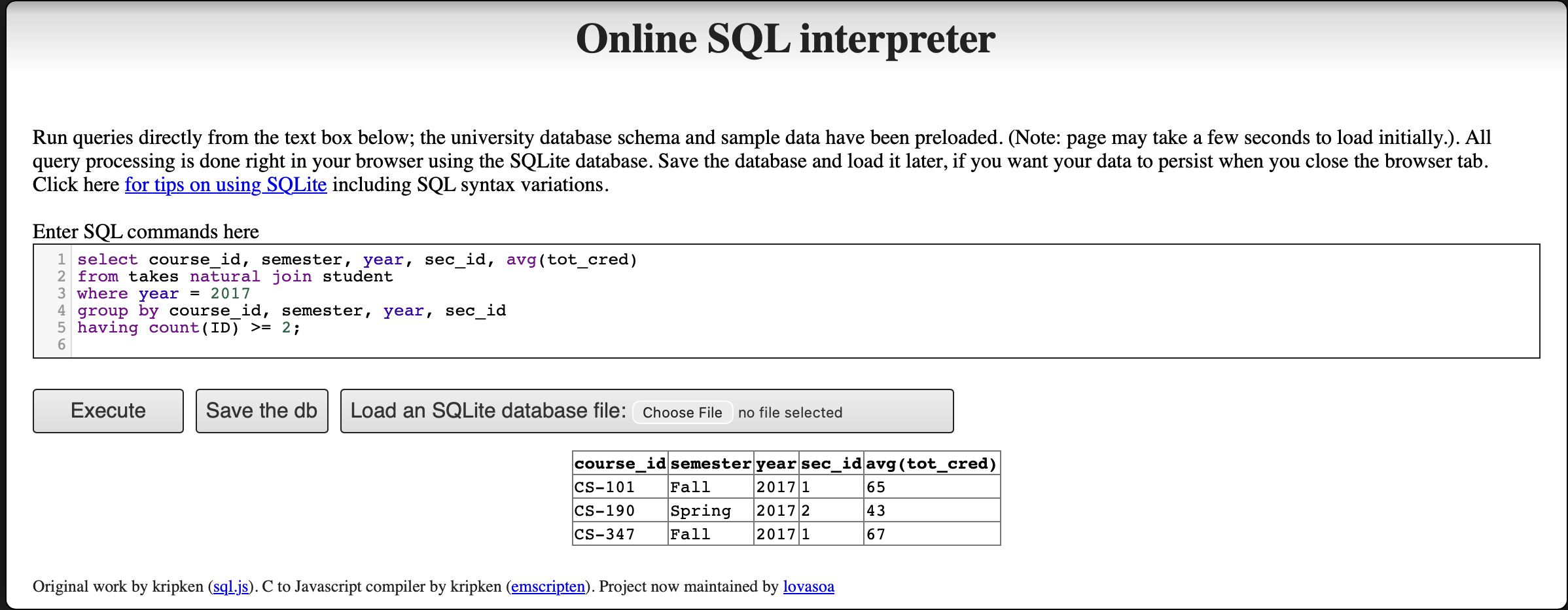
Consider the following query:

select course_id, semester, year, sec_id, avg (tot_cred)
from takes natural join student
where year = 2017
group by course_id, semester, year, sec_id
having count (ID) >= 2;

i. Explain why appending natural join section in the from clause would not change the result.

The relation takes already contains the attributes (course_id, sec_id, semester, year), which together form the primary key of the section relation. Because of the foreign key constraint from takes to section, every tuple in takes is guaranteed to have a matching tuple in section.

Therefore, adding natural join section to the from clause is a lossless join:

No rows are added, because each tuple in takes matches at most one tuple in section (since the join is on the primary key of section).
No rows are removed, because every tuple in takes has a corresponding tuple in section (due to the foreign key constraint).

The only effect of the additional join is that extra attributes from section (such as building, room_number, and time_slot_id) are appended to each tuple. However, since these attributes do not appear in the select, where, group by, or having clauses, they have no impact on the query result. The output remains identical.

ii. Test the results using the Online SQL interpreter.

Without natural join section:

With natural join section appended:

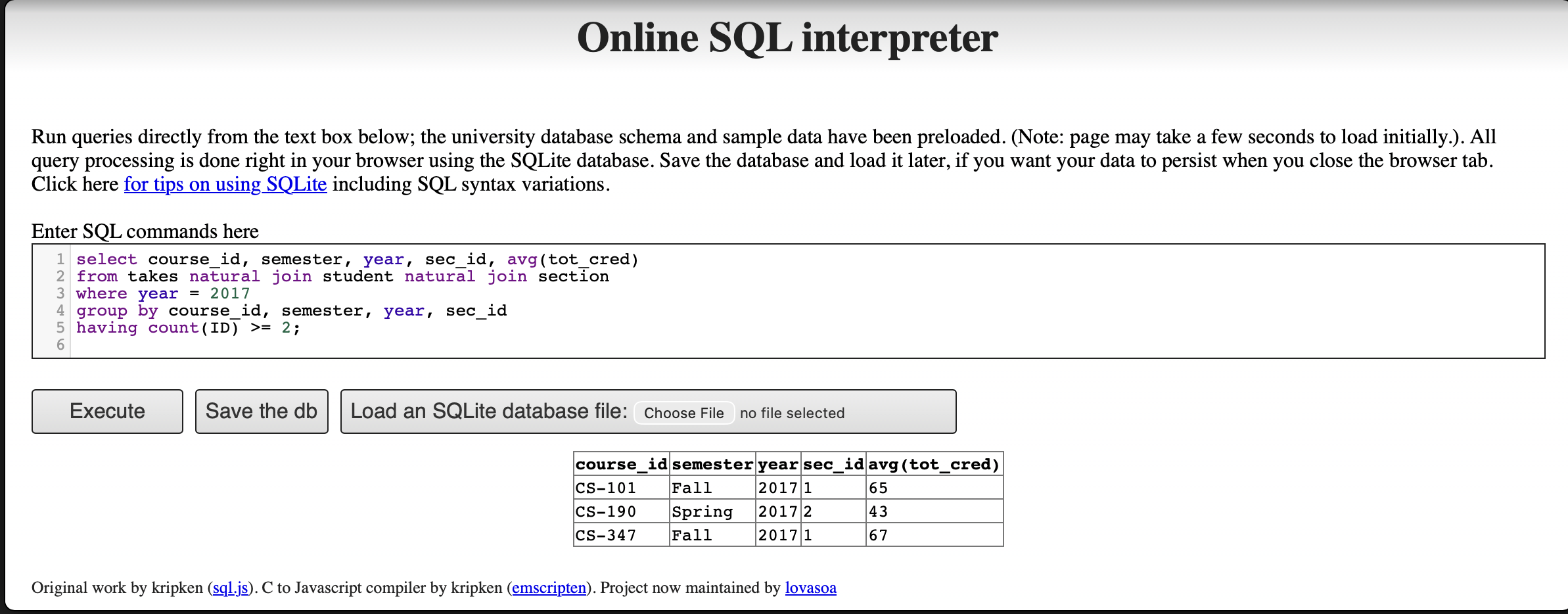
Both queries return identical results (CS-101, CS-190, CS-347), confirming that appending natural join section does not change the output.

3b

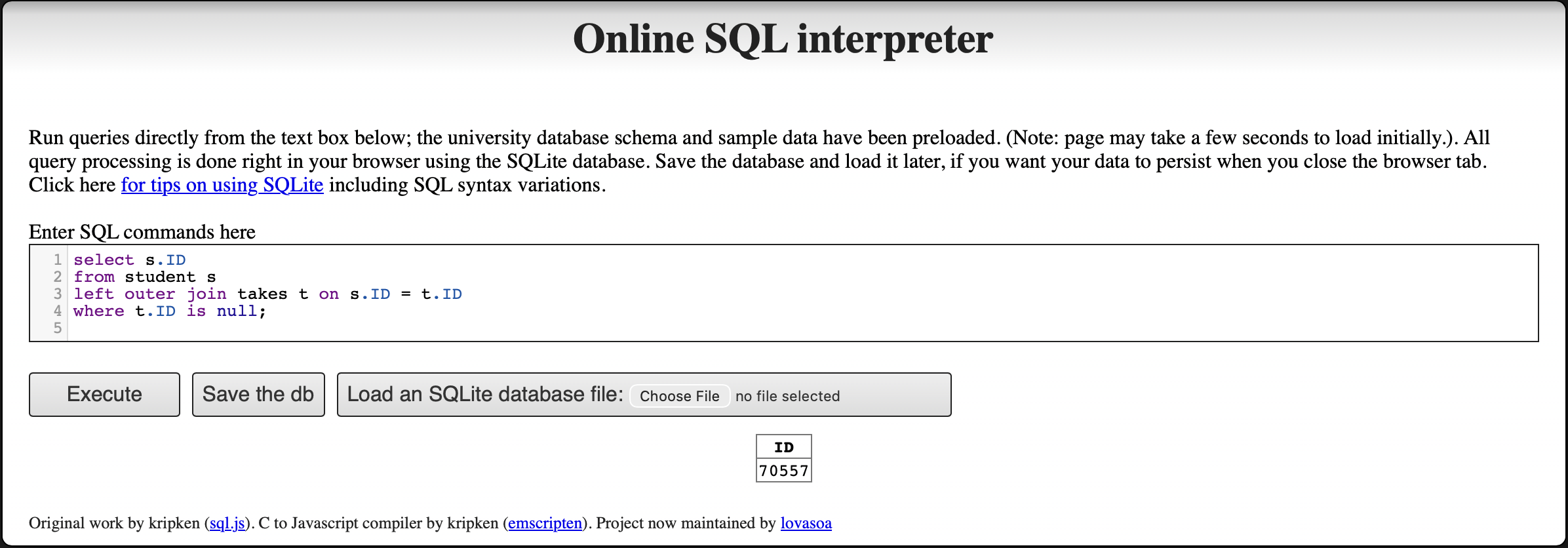
Write an SQL query using the university schema to find the ID of each student who has never taken a course at the university. Do this using no subqueries and no set operations (use an outer join). (Consult Ch. 4, 4.1.3)

select s.ID
from student s
left outer join takes t on s.ID = t.ID
where t.ID is null;

The left outer join preserves every tuple from the student relation. For students who have no matching record in takes (i.e., they have never enrolled in any course), all attributes from takes are filled with null. The where t.ID is null condition filters the result to include only those students whose ID has no match in takes, meaning they have never taken any course.

This approach avoids subqueries and set operations by leveraging the property of outer joins: unmatched rows from the preserved (left) side produce null values on the non-preserved (right) side, which can then be detected with an is null test.

Q3b — Students who have never taken a course

Assignment 5

Question 1

An E-R diagram can be viewed as a graph. What do the following mean in terms of the structure of an enterprise schema?

a) The graph is disconnected

In graph theory, a disconnected graph means the graph has at least two connected components — that is, there exist nodes with no path between them. In the context of an enterprise E-R schema, this means the diagram contains at least two groups of entity sets and relationship sets that are completely independent of each other, sharing no relationships, no foreign key references, and no common attributes. In practice, this implies the schema is modeling two or more entirely separate business domains with no interaction between them.

b) The graph has a cycle

In graph theory, a cycle means there exist two nodes in the graph that are connected by two or more completely distinct paths. In the context of an enterprise E-R schema, this means there are multiple relationship paths connecting the same set of entity sets.

However, a cycle does not necessarily imply redundancy. Each path in the cycle may carry semantically independent information — for example, one path may capture relationship attributes along the x-dimension and another along the y-dimension, and neither can be derived from the other. Whether the cycle represents true redundancy depends entirely on the semantic constraints of the domain: a relationship is truly redundant only if its information can be fully derived from the other paths in the cycle. Therefore, a cycle signals complex interdependencies in the schema that require careful analysis, but not automatic redundancy.

Question 3

We can convert any weak entity set to a strong entity set by simply adding appropriate attributes. Why, then, do we have weak entity sets?

Although it is technically possible to convert any weak entity set to a strong entity set by adding a unique identifier attribute (e.g., a surrogate key), weak entity sets are still useful and preferred for the following reasons:

Semantic Clarity and Modeling Fidelity. Weak entity sets reflect genuine real-world dependencies. For example, a room within a building only has meaning relative to the building it belongs to. Converting it into a strong entity set by assigning a globally unique room_id would technically work, but would obscure this inherent dependency and make the schema harder to understand.
Avoiding Meaningless Surrogate Keys. Creating unique keys for entities that have no independent identity — such as order items within an order, or a patient’s log entries within a hospital — forces the introduction of artificial keys that carry no real-world meaning. This adds complexity without improving the quality of the data model.
Enforcing Referential Integrity and Existence Dependency. Weak entity sets make existence dependencies explicit in the schema. Because a weak entity set can only exist if its identifying (owner) entity exists, this constraint is built into the model. If the owner entity is deleted, its dependent weak entities are automatically considered invalid. This enforces data integrity at the conceptual level in a way that a strong entity set with a foreign key constraint does not as clearly communicate.
Reducing Redundancy. If a weak entity’s natural identifier is only unique within the context of its owner (e.g., section number within a course), using a composite identifier (owner key + discriminator) is more compact and meaningful than introducing an entirely new global key. It avoids duplicating the owner’s key information unnecessarily.

In summary, weak entity sets improve the expressiveness and clarity of the E-R model. They allow designers to accurately represent entities whose existence and identity are inherently tied to another entity, leading to schemas that are easier to understand, maintain, and reason about.

Question 4

4a

Consider the employee database:

employee (ID, person_name, street, city)
works (ID, company_name, salary)
company (company_name, city)
manages (ID, manager_id)

where the primary keys are underlined. Give an expression in SQL for each of the following queries.

i. Find ID and name of each employee who lives in the same city as the location of the company for which the employee works.

SELECT e.ID, e.person_name
FROM employee AS e, works AS w, company AS c
WHERE e.ID = w.ID
  AND w.company_name = c.company_name
  AND e.city = c.city;

This query joins employee with works to link each employee to their company, then joins with company to get the company’s city. The WHERE clause then filters for employees whose city matches the city of their employer.

ii. Find ID and name of each employee who lives in the same city and on the same street as does her or his manager.

SELECT e.ID, e.person_name
FROM employee AS e, manages AS m, employee AS mgr
WHERE e.ID = m.ID
  AND m.manager_id = mgr.ID
  AND e.city = mgr.city
  AND e.street = mgr.street;

This query uses the manages table to identify each employee’s manager, then joins employee twice — once for the employee (aliased as e) and once for the manager (aliased as mgr). The WHERE clause requires both the city and the street to match between the employee and their manager.

iii. Find ID and name of each employee who earns more than the average salary of all employees of her or his company.

SELECT e.ID, e.person_name
FROM employee AS e, works AS w
WHERE e.ID = w.ID
  AND w.salary > (
    SELECT AVG(w2.salary)
    FROM works AS w2
    WHERE w2.company_name = w.company_name
  );

This query uses a correlated subquery to compute, for each employee, the average salary of all employees at their company. The outer query then filters for employees whose salary exceeds this per-company average. The correlation is established by matching w2.company_name = w.company_name.

4b

Consider the following SQL query that seeks to find a list of titles of all courses taught in Spring 2017 along with the name of the instructor.

SELECT name, title
FROM instructor NATURAL JOIN teaches
     NATURAL JOIN section NATURAL JOIN course
WHERE semester = 'Spring' AND year = 2017

What is wrong with this query?

The problem lies in how NATURAL JOIN works: it joins on all columns that share the same name across the joined relations. In the standard university schema, the relations have the following attributes:

instructor(ID, name, dept_name, salary)
teaches(ID, course_id, sec_id, semester, year)
section(course_id, sec_id, semester, year, building, room_number, time_slot_id)
course(course_id, title, dept_name, credits)

When the query performs instructor NATURAL JOIN teaches, it correctly joins on ID. When it then joins with section, it correctly joins on course_id, sec_id, semester, year. However, when it finally joins with course, both the running result (from instructor) and course contain the attribute dept_name. The NATURAL JOIN therefore additionally enforces the condition instructor.dept_name = course.dept_name, which incorrectly restricts the results to only include cases where the instructor belongs to the same department as the course.

This is incorrect because instructors can — and often do — teach courses offered by departments other than their own. Those cross-department teaching assignments would be wrongly excluded from the query results.

The fix is to replace only the last NATURAL JOIN course with an explicit JOIN course USING (course_id). This ensures that the join with course is performed only on course_id, preventing dept_name from being silently included as a join condition:

SELECT name, title
FROM instructor NATURAL JOIN teaches
     NATURAL JOIN section
     JOIN course USING (course_id)
WHERE semester = 'Spring' AND year = 2017;

This version controls exactly which attribute is joined on, preventing dept_name from unintentionally filtering out cross-department teaching assignments.

Assignment 6

Question 1 — Websites Using JSON and XML

Look up websites containing the following data representations: a) Using JSON, b) Using XML. Analyze the websites in terms of structure and composition. Name the technology/methods use for creating the web database.

a) JSON Example — GitHub API User Data

URL: https://api.github.com/users/octocat

This page shows public GitHub user data in JSON format. The data is returned as a JSON object with many key-value pairs such as login, id, html_url, followers, and created_at.

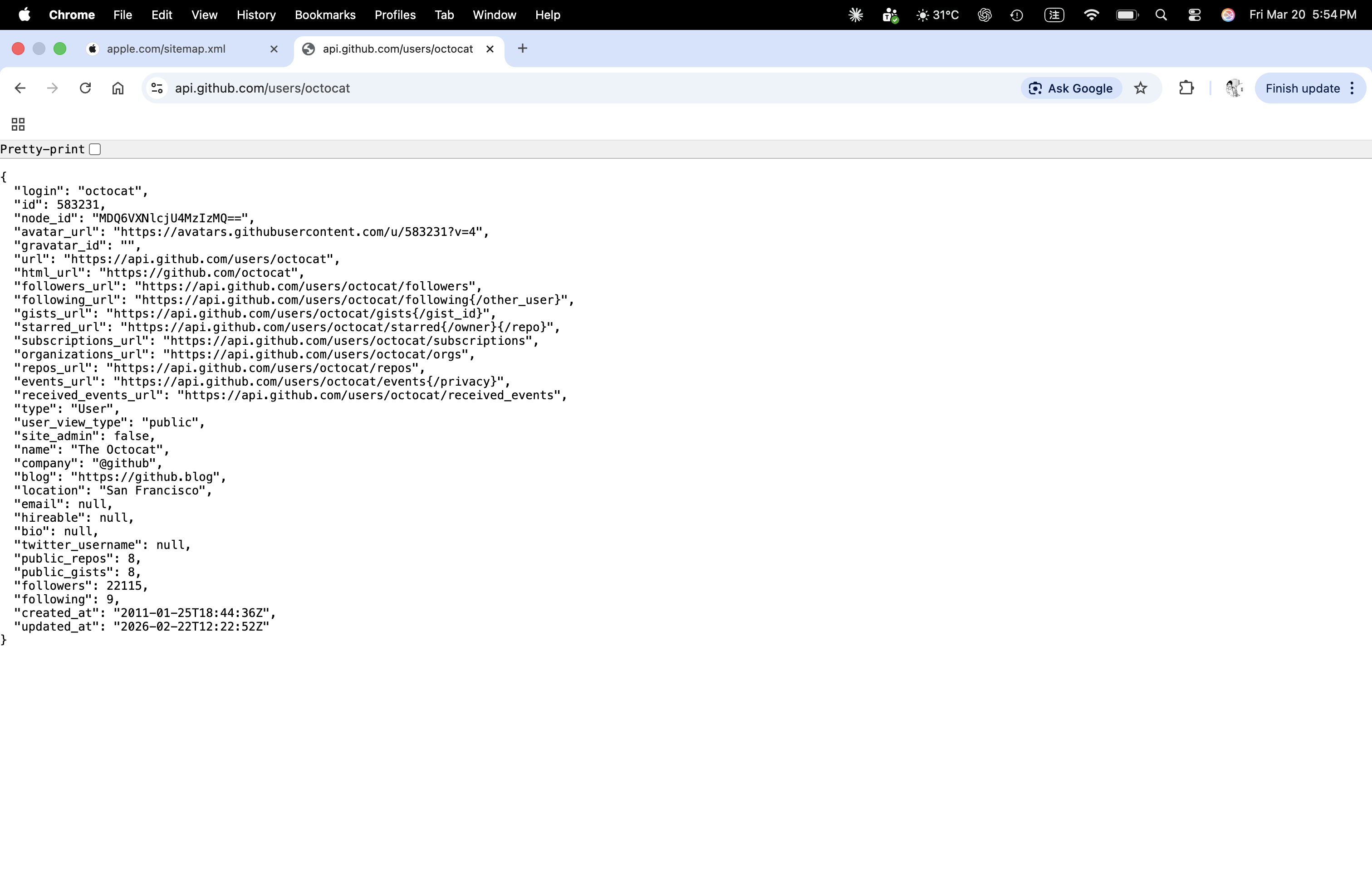
GitHub API JSON response for user octocat

Structure and composition:

The outer structure is a JSON object marked by { }.
Each field is stored as a key-value pair, for example "login": "octocat".
The response contains strings, numbers, URLs, boolean values, and null values.
This format is lightweight and easy for websites and apps to exchange data.

Possible technologies / methods:

REST API
Backend web service
Database support such as PostgreSQL, MySQL, or NoSQL systems
JSON response for web and application data exchange

b) XML Example — Apple Sitemap

URL: https://www.apple.com/sitemap.xml

This page shows Apple’s sitemap in XML format. It lists webpage links so that search engines can discover and index the site.

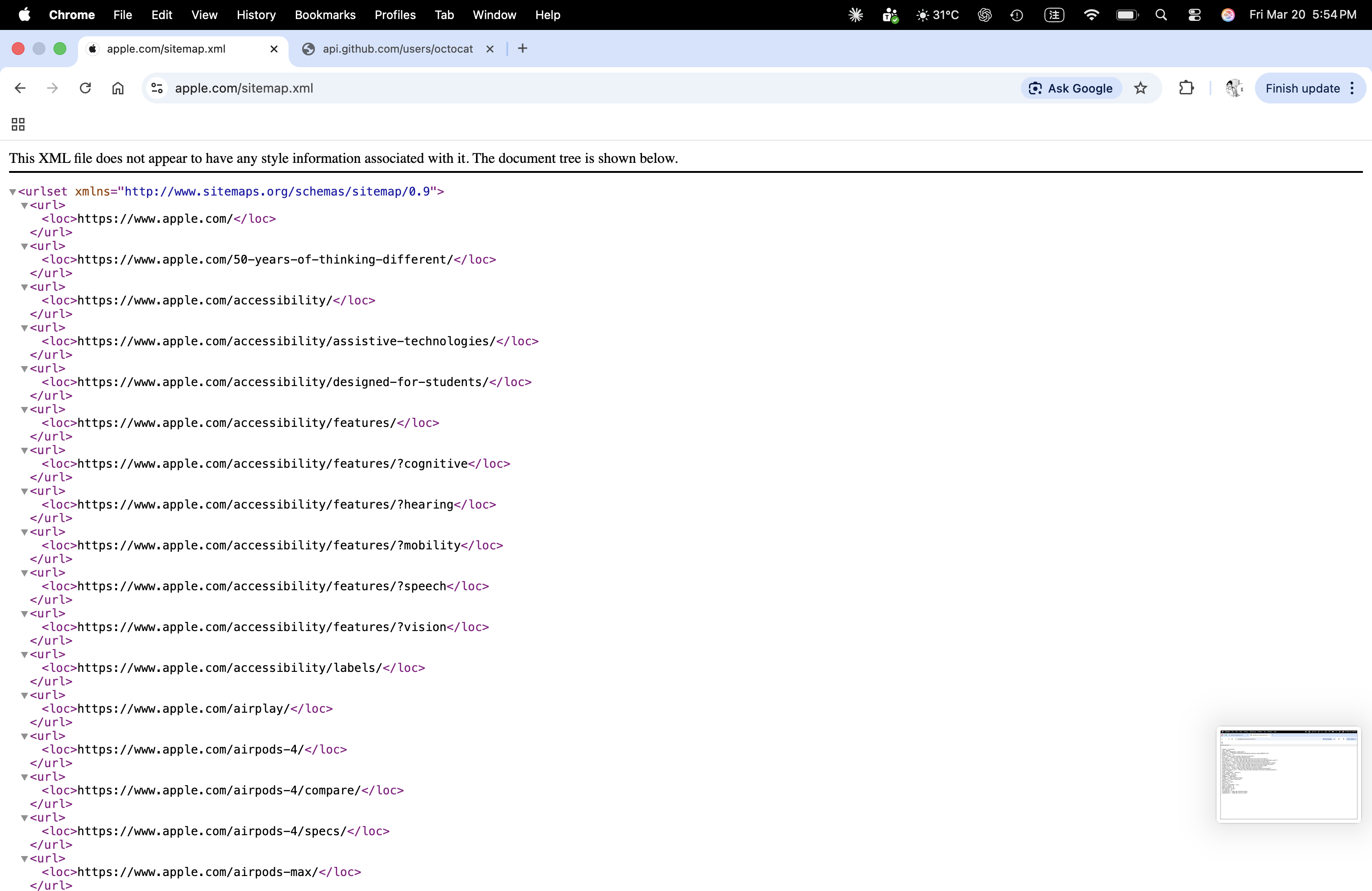
Structure and composition:

The root element is <urlset>.
Each webpage entry is stored inside a repeated <url> element.
The actual page address is stored inside the <loc> tag.
The data is organized in a hierarchical tag structure, which is a key feature of XML.

Possible technologies / methods:

XML sitemap standard
Website content publishing system or CMS
Backend-generated data from a site database
Search engine indexing support

Quick Comparison

JSON is shorter and easier for web APIs and applications.
XML uses tags and hierarchy, so it is useful for structured documents and sitemaps.
Both formats help websites store or exchange data in an organized way.

Question 2 — SQL Exercises

i. Students Without Advisors (Left Outer Join)

Express the following query in SQL using no subqueries and no set operations. (Hint: left outer join)

select ID
from student
except
select s_id
from advisor
where i_ID is not null

Idea: Keep all rows from student by using LEFT OUTER JOIN. Match student.ID with advisor.s_id. If a student has no matching advisor row, then advisor columns become NULL. Therefore, where a.s_id is null returns students without advisors.

SQL answer:

select s.ID
from student s
left outer join advisor a
  on s.ID = a.s_id
where a.s_id is null;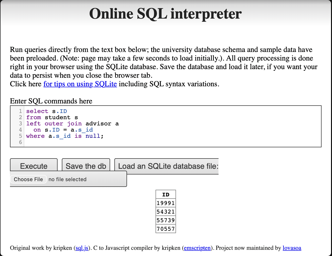

Q2i — Students without advisors using LEFT OUTER JOIN

ii. Instructors Who Teach Every Course in Their Department

Using the university schema, write an SQL query to find the names and IDs of those instructors who teach every course taught in his or her department (i.e., every course that appears in the course relation with the instructor’s department name). Order result by name.

Idea: For each instructor, first limit the scope to courses in the same department. Then check whether there exists any department course that the instructor did not teach. If no such course exists, then the instructor taught every course in the department. This is why the query uses NOT EXISTS with another NOT EXISTS inside it.

SQL answer:

select i.name, i.ID
from instructor i
where not exists (
    select *
    from course c
    where c.dept_name = i.dept_name
      and not exists (
          select *
          from teaches t
          where t.ID = i.ID
            and t.course_id = c.course_id
      )
)
order by i.name;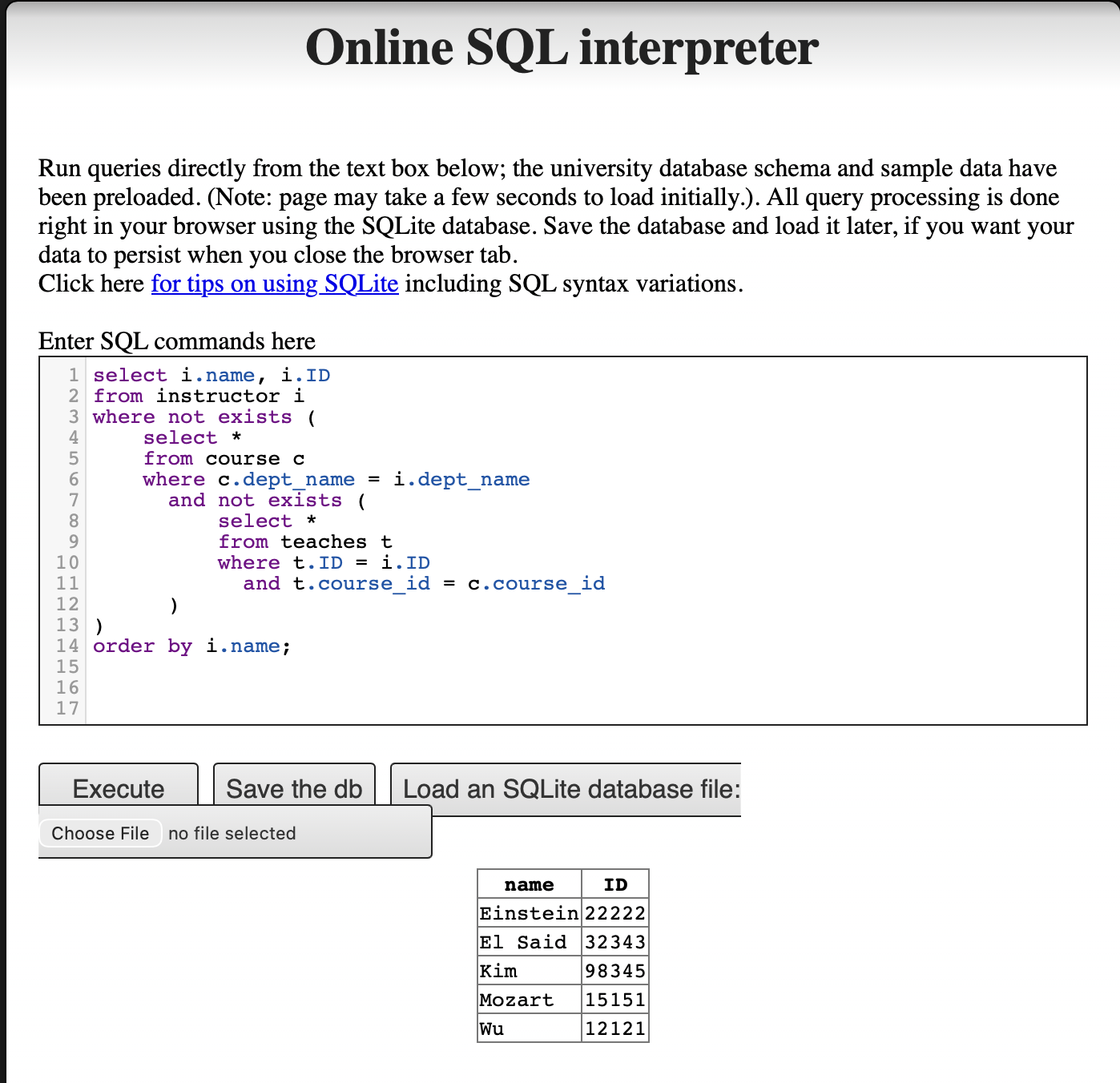

Q2ii — Instructors who teach every course in their department

Question 3 — R and PostgreSQL

a) Import the Full Database

The university database was created using the DDL (Data Definition Language) schema and populated with the large relations insert file from the textbook website.

DDL schema (DDL.sql):

create table classroom
    (building       varchar(15),
     room_number    varchar(7),
     capacity       numeric(4,0),
     primary key (building, room_number)
    );

create table department
    (dept_name      varchar(20),
     building       varchar(15),
     budget         numeric(12,2) check (budget > 0),
     primary key (dept_name)
    );

create table course
    (course_id      varchar(8),
     title          varchar(50),
     dept_name      varchar(20),
     credits        numeric(2,0) check (credits > 0),
     primary key (course_id),
     foreign key (dept_name) references department (dept_name)
        on delete set null
    );

create table instructor
    (ID             varchar(5),
     name           varchar(20) not null,
     dept_name      varchar(20),
     salary         numeric(8,2) check (salary > 29000),
     primary key (ID),
     foreign key (dept_name) references department (dept_name)
        on delete set null
    );

create table section
    (course_id      varchar(8),
     sec_id         varchar(8),
     semester       varchar(6)
        check (semester in ('Fall', 'Winter', 'Spring', 'Summer')),
     year           numeric(4,0) check (year > 1701 and year < 2100),
     building       varchar(15),
     room_number    varchar(7),
     time_slot_id   varchar(4),
     primary key (course_id, sec_id, semester, year),
     foreign key (course_id) references course (course_id)
        on delete cascade,
     foreign key (building, room_number) references classroom
        on delete set null
    );

create table teaches
    (ID             varchar(5),
     course_id      varchar(8),
     sec_id         varchar(8),
     semester       varchar(6),
     year           numeric(4,0),
     primary key (ID, course_id, sec_id, semester, year),
     foreign key (course_id, sec_id, semester, year)
        references section on delete cascade,
     foreign key (ID) references instructor (ID)
        on delete cascade
    );

create table student
    (ID             varchar(5),
     name           varchar(20) not null,
     dept_name      varchar(20),
     tot_cred       numeric(3,0) check (tot_cred >= 0),
     primary key (ID),
     foreign key (dept_name) references department (dept_name)
        on delete set null
    );

create table takes
    (ID             varchar(5),
     course_id      varchar(8),
     sec_id         varchar(8),
     semester       varchar(6),
     year           numeric(4,0),
     grade          varchar(2),
     primary key (ID, course_id, sec_id, semester, year),
     foreign key (course_id, sec_id, semester, year)
        references section on delete cascade,
     foreign key (ID) references student (ID)
        on delete cascade
    );

create table advisor
    (s_ID           varchar(5),
     i_ID           varchar(5),
     primary key (s_ID),
     foreign key (i_ID) references instructor (ID)
        on delete set null,
     foreign key (s_ID) references student (ID)
        on delete cascade
    );

create table time_slot
    (time_slot_id   varchar(4),
     day            varchar(1),
     start_hr       numeric(2) check (start_hr >= 0 and start_hr < 24),
     start_min      numeric(2) check (start_min >= 0 and start_min < 60),
     end_hr         numeric(2) check (end_hr >= 0 and end_hr < 24),
     end_min        numeric(2) check (end_min >= 0 and end_min < 60),
     primary key (time_slot_id, day, start_hr, start_min)
    );

create table prereq
    (course_id      varchar(8),
     prereq_id      varchar(8),
     primary key (course_id, prereq_id),
     foreign key (course_id) references course (course_id)
        on delete cascade,
     foreign key (prereq_id) references course (course_id)
    );

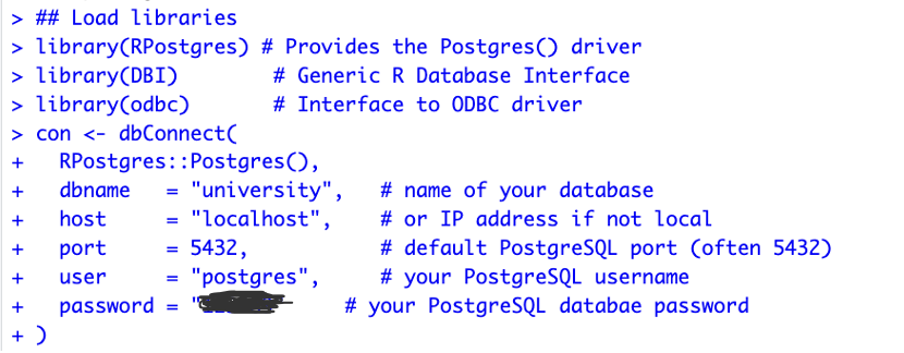
b) Run RPostgres01.R

The R script connects to the local PostgreSQL database using RPostgres and DBI, runs three queries, exports a CSV, and disconnects.

Load libraries and connect:

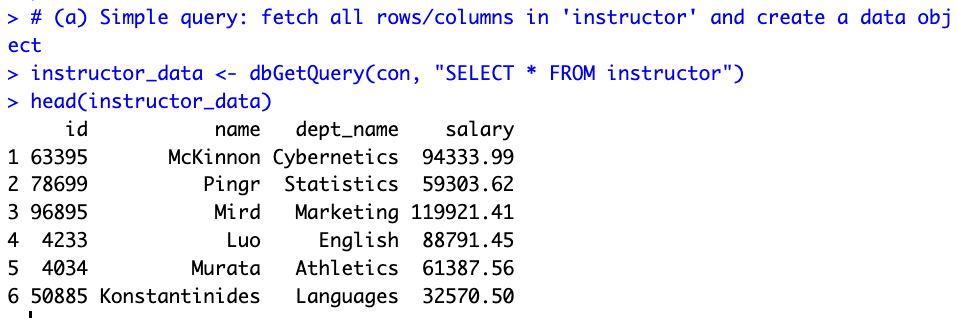
Query (a) — Fetch all instructors:

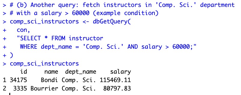
Query (b) — Comp. Sci. instructors with salary > 60000:

R — Comp. Sci. instructors with salary > 60000

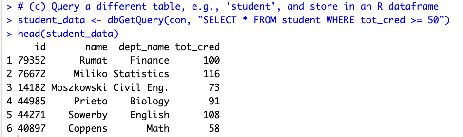
Query (c) — Students with tot_cred >= 50:

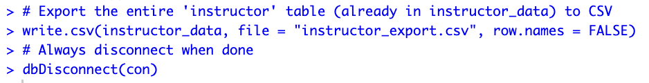
Export to CSV and disconnect:

R — Export instructor table to CSV and disconnect

c) Results

R script (RPostgres01.R):

# Connect PostgreSQL database using R
# Packages: DBI, odbc, RPostgres
# Documentation:
## DBI: https://dbi.r-dbi.org
## RPostgres https://github.com/r-dbi/RPostgres
## R https://solutions.posit.co/connections/db/
## odbc: https://solutions.posit.co/connections/db/best-practices/drivers/

install.packages(c("RPostgres", "DBI", "odbc"))

## Load libraries
library(RPostgres)
library(DBI)
library(odbc)

## Connect to PostgreSQL and database
con <- dbConnect(
  RPostgres::Postgres(),
  dbname   = "university",
  host     = "localhost",
  port     = 5432,
  user     = "postgres",
  password = "123489"
)

## Perform queries

# (a) Simple query: fetch all rows/columns in 'instructor'
instructor_data <- dbGetQuery(con, "SELECT * FROM instructor")
head(instructor_data)

# (b) Fetch instructors in 'Comp. Sci.' department with salary > 60000
comp_sci_instructors <- dbGetQuery(
  con,
  "SELECT * FROM instructor
   WHERE dept_name = 'Comp. Sci.' AND salary > 60000;"
)
comp_sci_instructors

# (c) Query 'student' table: students with tot_cred >= 50
student_data <- dbGetQuery(con, "SELECT * FROM student WHERE tot_cred >= 50")
head(student_data)

## Export to CSV
write.csv(instructor_data, file = "instructor_export.csv", row.names = FALSE)

## Clean up
dbDisconnect(con)

Assignment 7 — AI Exercise (Shiny)

Two Shiny apps were built, modified according to the assignment requirements, and deployed live to shinyapps.io. App 1 was re-engineered from a local PostgreSQL connection to a bundled SQLite database so that it runs fully in the cloud without requiring the instructor’s machine to host a server.

App 1 — University Database (SQLite + ggplot2)

Modifications applied:

(a) Password / connection. The original RPostgres connection to localhost:5432 was replaced with a file-based SQLite connection: dbConnect(RSQLite::SQLite(), "university.db"). The university.db file was built from the textbook’s DDL.sql and largeRelationsInsertFile.sql and bundled with the app.
(b) Sort salary high → low. Changed reorder(dept_name, y_value) to reorder(dept_name, -y_value) so the tallest bar sits on the left.
(c) Another variable from another table. Added a selectInput dropdown that switches between two queries: average instructor salary (table instructor) and average student total credits (table student).

Live app: https://chentzuyuan.shinyapps.io/epps6354-hw7-1/

App 2 — Old Faithful Geyser Histogram

Modification applied:

(a) Barchart color. Changed col = "blue" to the project’s global palette — fill #18A3A380 (teal, color1), border #FF4D8DCC (pink, color2) — for consistency with App 1.

Live app: https://chentzuyuan.shinyapps.io/epps6354-hw7-2/

Assignment 8 — NBA Database Shiny App

Following the workshop at datageneration/informationmanagement — workshop/Shiny, the full pipeline was reproduced end-to-end and deployed live to shinyapps.io.

a) Build the NBA database on local PostgreSQL

The course-provided NBAPlayers.sql file was loaded into a fresh PostgreSQL 18 database named NBAplayers:

createdb -U postgres NBAplayers
psql -U postgres -d NBAplayers -f NBAPlayers.sql

Three tables were populated: player (4,501 rows), player_salary (1,292 rows), and player_photos (4,593 rows).

b) Export into SQLite

Because the SQL file’s CREATE TABLE syntax is already SQLite-friendly, the same file was loaded directly into a SQLite database file nba.db — no manual schema translation was needed:

sqlite3 nba.db < NBAPlayers.sql

Row counts in nba.db exactly match the PostgreSQL build (4,501 / 1,292 / 4,593), confirming a clean export.

c) Embed in Shiny

The app follows the instructor-provided template structure: a single slider that controls how many active players to render in a DT DataTable, with each row’s headshot embedded as an <img> tag.

The query inner-joins Player with Player_Photos on idPlayer and filters to is_active = 1:

SELECT p.id, p.first_name, p.last_name, p.full_name,
       pp.urlPlayerHeadshot
FROM Player p
INNER JOIN Player_Photos pp ON pp.idPlayer = p.id
WHERE p.is_active = 1
LIMIT <slider_value>;

The headshot column is rendered with escape = FALSE so the URLs become inline images:

table_df$headshot <- paste0(
  '<img src="', table_df$urlPlayerHeadshot, '"></img>'
)

The same color palette as Assignment 7 (#18A3A380 header, #FF4D8DCC border) is applied via custom CSS so the look matches the rest of the site.

d) Deploy on Shinyapps.io

rsconnect::deployApp(
  appDir   = "nba-shiny",
  appName  = "epps6354-hw8-nba",
  appFiles = c("app.R", "nba.db")
)

The nba.db SQLite file is bundled with the app, so the deployed instance is fully self-contained — no remote database connection needed.

Live app: https://chentzuyuan.shinyapps.io/epps6354-hw8-nba/

Final Report

Final Report Paper (PDF) → Live demo →

1. Project Overview

OutfitDB is a personalized outfit recommendation system. It stores the user’s wardrobe data, actual wear logs, and preference ratings on three independent axes (temperature, aesthetic, occasion) in a 13-table relational database. Three XGBoost classifiers are trained on top of this database, and their outputs are combined multiplicatively to produce daily Top-K outfit recommendations.

Unlike typical fashion apps that rely on dress-code templates or fixed style rules, OutfitDB’s recommendations evolve with the user’s ratings and wear feedback — the system does not tell the user what looks good, but learns what the user thinks looks good.

The product ships in two forms: a desktop application packaged with PyInstaller for macOS / Windows (the primary product), and a public web trial hosted on Render. Each user corresponds to an independent SQLite file under the local-first design — data never leaves the user’s machine.

Current release: v0.3.1 (May 2026). Architecture: 13 tables, 3 XGBoost classifiers, four-stage multiplicative scoring. Scale: ~2,000 lines of Python on the backend; ~3,000 lines of vanilla JS / HTML / CSS on the frontend.

2. Technology Stack

Layer	Technology	Purpose
Backend	FastAPI (Python 3.12)	HTTP routing, async support, Pydantic
ORM	SQLAlchemy 2.x	Object-relational mapping
Database	SQLite	Embedded relational DB; one file per user
Frontend	Vanilla HTML / CSS / JS	No build step (no React)
Charts	Chart.js 4.4 (CDN)	Stats dashboard + per-item modal
ML	XGBoost	Three independent gradient-boosted classifiers
Migrations	create_all + idempotent ALTER	No Alembic
Hosting (web)	Render.com	uvicorn + persistent disk for SQLite
Packaging	PyInstaller	Cross-platform .dmg / .exe
Style sharing	.odstyle JSON	Trained model exported as a portable file

The stack was not planned in full upfront; it took shape through iterative adjustment.

2.1 Backend: Shiny → FastAPI

The first deployment used R Shiny — the original public URL is preserved at the original Shiny version (named ClosetMind at that stage; kept to illustrate the prototype phase, in which several functions could not run reliably on Shiny).

Three concrete pain points emerged in production:

File upload was awkward — the lifecycle of multi-photo validation, resizing, on-disk storage, and linking to a DB row falls outside Shiny’s design space.
Cross-page state management was difficult — Shiny’s reactive model is not well suited to a multi-page workflow such as upload → tag → wear → train → recommend.
ML inference blocked the R session — XGBoost calls would tie up R workers.

The backend was rewritten in FastAPI + uvicorn and deployed on Render.

2.2 Database: PostgreSQL → SQLite

The first version of the database was built on PostgreSQL. The schema was designed against my personal wardrobe; additional clothing items were later added manually to broaden the demo dataset, and some clothing photographs were generated with DALL-E because the photographic environment was constrained.

During deployment, PostgreSQL’s requirement for a separate DB server conflicted with the local-first product positioning. The data was therefore exported from PostgreSQL and migrated to SQLite, with each user mapped to an independent file.

2.3 ML: XGBoost (chosen from the outset)

Training data is small tabular data (typically fewer than 5,000 ratings per user). Gradient boosting outperforms neural networks at this scale (Grinsztajn et al., NeurIPS 2022). Inference latency is low and the model is interpretable (feature importance, SHAP).

2.4 Frontend: HTML/CSS → Vanilla JS

The frontend was initially written in HTML and CSS only. As the feature set grew (dynamic lists, real-time updates, AJAX with the backend, recommendation interactivity), pure HTML and CSS were no longer sufficient. After research, vanilla JavaScript was added rather than React — the application is small (5–10 pages), build-step complexity (Vite / webpack / npm dependencies) is avoided, initial load is faster, and the learning curve is gentler.

3. Overall Architecture

OutfitDB’s data flow consists of three writers feeding a central database, three classifiers reading from the database, and one recommendation engine.

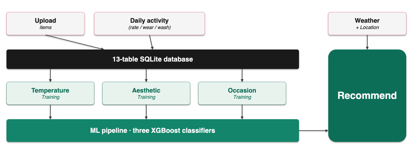
Three writers

Upload — one-time wardrobe registration (uploading clothing photos and attributes).
Daily activity — continuous writes (rating, marking worn, marking washed).
Weather + Location — real-time fetch, not persisted to the DB; fed directly into the recommendation engine.

Three training pipelines

Training data read from the database feeds three classifiers respectively — Stage 1 temperature, Stage 2 aesthetic, Stage 3 occasion.

4. Database Schema (13 tables, 5 clusters)

The schema is designed in 3NF, with deliberate denormalizations only at three documented locations (see §5).

4.1 Cluster A — Wardrobe Identity (3 tables)

Static identity data describing what the user owns.

users — one SQLite file ↔︎ one user, but user_id is retained as a forward-looking field for future N:M style sharing. Key fields: id, display_name, lat, lon, temp_offset, training_complete, has_thermal_insoles, created_at.
items — one row per clothing item, ~30 fields grouped by identification, structure, visual, material, category-specific, and operations. Soft delete via is_active.
item_tags — open key-value metadata for attributes not anticipated upfront (e.g., brand, purchase_date). UniqueConstraint(item_id, key, value) prevents duplicates.

4.2 Cluster B — Lifecycle Partitioning (2 tables)

Embodies the principle of partitioning by access frequency (see §5.1). The fields of a single clothing item are split into two 1:1-related smaller tables based on write frequency.

item_states — hot-write region; every wear / wash event triggers an UPDATE. Fields: state, worn_count, wear_count_since_wash, last_worn.
item_stats — aggregate cache region; recomputed lazily after rating events. Fields: coverage_count, total_ratings, average_rating, last_worn_date, days_since_worn.

4.3 Cluster C — Outfits & Contexts (3 tables)

outfits — one outfit, composed of multiple items. Fields: warmth_score, coverage_curve, aesthetic_curve, optimal_layer_count, overkill_layers, aesthetic_stop_layers, underfit_flag.
outfit_items — M2M junction (outfit ↔︎ item).
daily_contexts — daily wearing context, kept as a separate table to avoid the transitive dependency outfit → context → date → weather. Fields: date, temperature, weather, humidity, wind, occasion, calendar_event.

4.4 Cluster D — Three Preference Axes (3 tables)

Each ML classifier has its own dedicated rating table (see §5.2).

ratings — Stage 2 aesthetic ratings, integer values −1 / 0 / 1 / 2. UniqueConstraint(user_id, outfit_id) plus an extra ideal_temp_zone.
temperature_ratings — Stage 1, JSON list of zones the outfit suits.
occasion_ratings — Stage 3, JSON list of events the outfit suits.

4.5 Cluster E — History & ML Provenance (2 tables)

outfit_logs — actual wear vs. system recommendation. Fields: recommended_outfit_id, final_worn_outfit_id, user_action (accepted / modified / rejected / skipped), scheduled_for, is_scheduled, logged_at. This table is the source of OutfitDB’s learning capability.
model_runs — audit trail of every model training run. The feature_version field gates .odstyle import compatibility.

5. Three Key Design Decisions

5.1 Decision 1 — Hot/Cold Vertical Partitioning

Problem. Putting every item field into a single table means every wear event rewrites the full ~1 KB row to disk, including columns such as colors and composition that did not change in 95% of cases.

Solution. Vertical partitioning — items (cold, edited monthly) / item_states (hot, edited daily) / item_stats (cache). Normalization addresses logical dependencies; partitioning addresses physical access — they operate at different layers of the design.

5.2 Decision 2 — One Rating Table per Classifier

Problem. A polymorphic super-table over different signal shapes (int vs. JSON list) introduces large numbers of NULL columns and forces every ML SELECT to filter on rating_kind.

Solution. Three concrete tables, one per classifier — clean type contracts, no NULL pollution, kind-free SELECTs. Polymorphism inside one table is debt; concrete tables are easier to reason about.

5.3 Decision 3 — Two Deliberate Denormalizations

The schema contains two intentional denormalizations, both motivated by performance:

Mirror the JSON. items.composition is a JSON list (blend ratios); items.material separately stores the highest-percentage fabric as an indexed VARCHAR. The mirror is set automatically from composition on insert and cannot drift.
Cache the join. item_stats.average_rating and coverage_count could in principle be computed by joining ratings × outfit_items; that join would run on every page load and degrade badly. Caching shifts the cost to write time via lazy updates on rating events.

The rest of the schema is BCNF-compliant.

6. ML Pipeline

Three independent XGBoost classifiers, integrated via multiplicative scoring, continuously refined by a feedback loop that learns the user’s personal style.

Stage	Name	Input features	Training source
1	Temperature classifier	Item features + current temp zone	`temperature_ratings`
2	Aesthetic classifier	Item features + outfit structure	`ratings`
3	Occasion classifier	Item features + current occasion	`occasion_ratings`

Multiplicative scoring

total = ctx_fit × stage1_pass × stage3_pass × aesthetic_blend

Multiplication (rather than addition) enforces that every dimension passes — if any single classifier is uncertain, the total score is pulled down. An outfit that is “aesthetically great but freezing” cannot survive this rule.

Feedback loop — the model tracks personal style

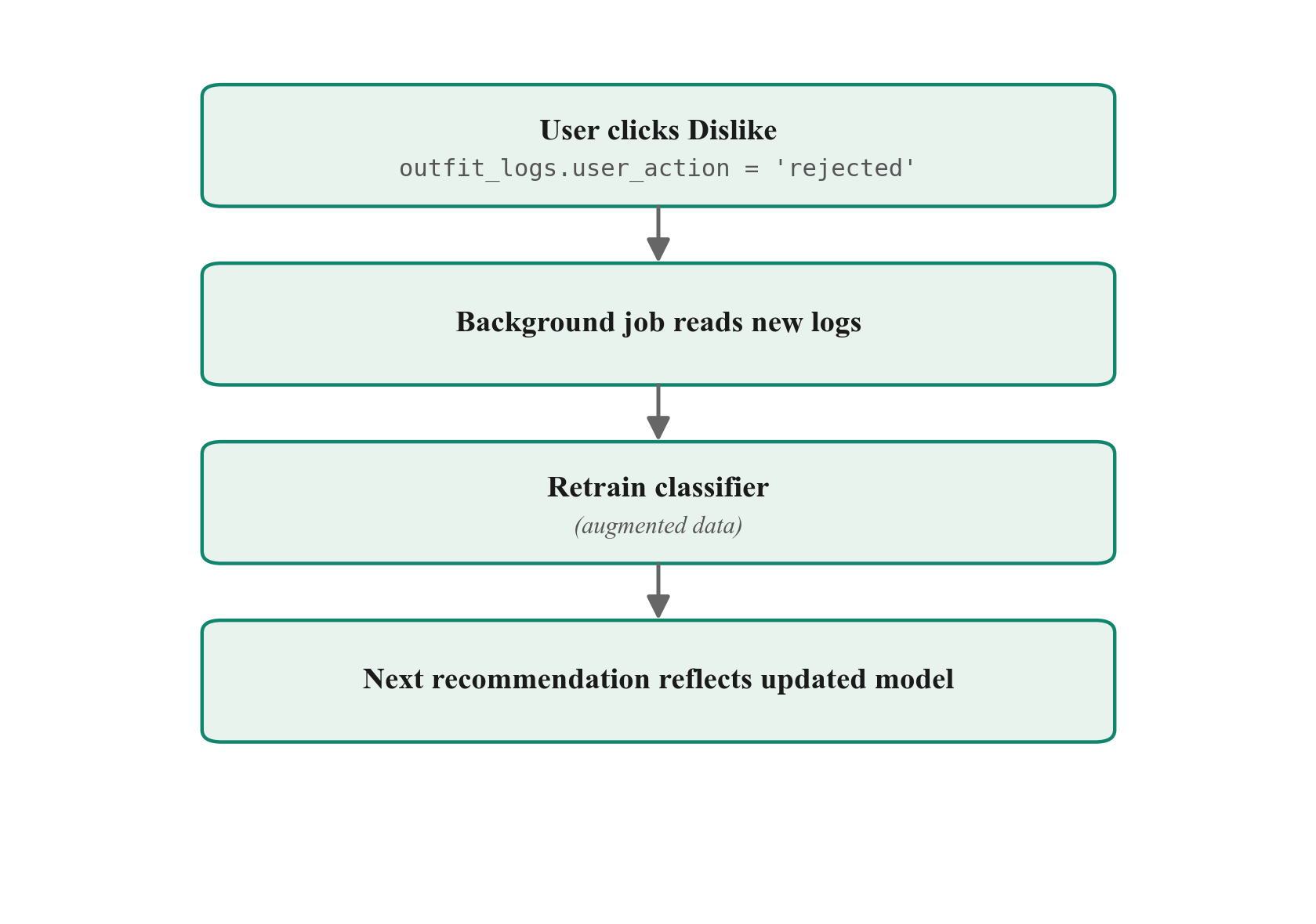
The outfit_logs table is the heart of this loop: it captures not only what the system recommended, but also what the user actually chose or rejected. As usage accumulates, the model gradually internalizes the user’s personal sense of style — under the same casual rock dress code, two different users will receive different outfits because each model has learned each individual’s preferences.

This is the central distinction between OutfitDB and a static dress-code template: the system does not tell the user what looks good — it learns what the user thinks looks good.

7. User Interface

Closet page — grid view with category / color / material / state filters and six sort modes. Clicking any item card opens a stats modal: 4 KPI tiles, wear timeline (13-week line chart), top-5 co-occurring items, and composition donut.
Stats dashboard — wardrobe-wide KPI tiles and six charts: items by category (doughnut), top 10 colors / materials (horizontal bar), aesthetic rating distribution, and most-worn / most-recommended top 10 (vertical bar). Page-level .odstyle export button.
Training UIs — three dedicated pages for the three ML axes: /training/temperature, /training/aesthetic, /training/occasion. Each axis must accumulate ≥6 batches of ratings before recommendations unlock.
Recommendation page — Top-K outfits with six per-card scores. Bold three (Aesthetic, Weather, Occasion) are the multiplicative ML axes; light gray three (Warmth, Freshness, Variety) are soft signals. Four sort modes are offered; sorting is client-side without re-querying the server.
Settings — personal preferences, imported .odstyle packs, and a manual Check for updates button (no automatic polling).
Internationalization (i18n) — bilingual UI via data-i18n attributes; the language toggle in the top-right corner switches between Chinese and English instantly without a page reload.

8. Deployment Architecture

8.1 Web demo (Render)

Platform: Render.com. Persistence via Render disk volume; SQLite files persist across deployments.
Cold start ~50 s on the free tier.
CI/CD: git push origin main → Render auto-deploy.
Public URL: https://outfitdb.onrender.com.

8.2 Desktop bundle (PyInstaller)

Targets: macOS .dmg / Windows .exe.
Contents: full Python runtime + uvicorn + all dependencies (single executable).
Data location: ~/Library/Application Support/OutfitDB/profiles/<name>/ on macOS.
Update check: manual — the Check for updates button on the Settings page fetches latest.json from a public GitHub raw URL.

8.3 Update manifest format

{
  "version":    "0.3.2",
  "url":        "https://github.com/.../OutfitDB-0.3.2.dmg",
  "update_url": "https://.../OutfitDB-0.3.2-update.zip",
  "full_url":   "https://.../OutfitDB-0.3.2-full.dmg",
  "notes":      "Adds X / fixes Y"
}

update_url (incremental update) and full_url (full installer) are both optional; url is a fallback for backwards compatibility.

9. Future Roadmap

9.1 Schema cleanup (paying down technical debt)

JSON arrays → M2M tables. items.colors and items.style_tags are currently JSON lists (violating 1NF); now that FEATURE_VERSION = 1 is locked, they can be refactored back into proper junction tables.
Remove last_worn duplication. Keep item_states.last_worn as the source of truth; compute item_stats.last_worn_date and days_since_worn at read time via Python @property.
Remove composition / material dual-write. Refactor material into a @property derived from composition, eliminating drift risk.
Items table inheritance. Trigger refactoring when categories exceed ten (items_base + items_top + items_bottom + ...).

9.3 Long-term — public style gallery

Extend .odstyle sharing into a public platform: users publish their own .odstyle files; others browse, preview, and try someone else’s model on their own wardrobe. OutfitDB does not sell clothes; it makes aesthetic taste the unit of exchange — measurable, portable, shareable.

10. AI Disclosure

AI assistance was used during the development of OutfitDB (Claude / Anthropic):

Code — authored by the author with Claude Code as a pair programmer.
Documentation, slides, and this report — drafted with Claude’s assistance; all schema design decisions, ML architecture choices, and final content were made by the author.

Translation note. The English version of the final paper was translated from the original Chinese manuscript using AI assistance (Claude / Anthropic), and was subsequently reviewed and revised by the author. Any translation errors that remain are the author’s responsibility.

Data Science · Applied Math · Machine Learning

"Bridging mathematical theory with data-driven solutions."

Projects

12+

Domains

Degrees

2.3M+

Max Data Processed

150x

Algorithm Speedup

Selected Projects

ResNet Image Classification

96.44% accuracy on multi-class classification with focal loss and transfer learning.

Deep Learning → 02

Distributed SVM with Nyström Approximation

150× speedup using 5-worker architecture with kernel approximation on large-scale datasets.

Big Data → 03

Medical Image Segmentation

U-Net and Conditional GAN for retinal vessel segmentation on biomedical imaging datasets.

Deep Learning → 04

Quantum Bayesian Inference

Undergraduate thesis investigating Bayesian probability on IBM quantum hardware using Qiskit.

Quantum Computing →

Ongoing Research

Flight Delay Prediction — M.S. Thesis

In Progress

Selective prediction framework for American Airlines flight delays. Investigating when not to trust model predictions by defining abstention policies that bound acceptable risk.

0.6863

AUC (No ETD)

0.9280

AUC (+ ETD)

0.2908

AURC

1.1M+

Flights

Data under NDA — results only, no raw data disclosed.

OutfitDB — Wardrobe Recommendation System

v0.2.0

Local-first desktop app that learns each user’s clothing preferences. Three-stage XGBoost pipeline (temperature × aesthetic × occasion) chained at inference time. Layer-coverage thermal model handles real cold-weather layering; auto-update notification ships from a public release feed. Final project for EPPS 6354 (Information Management).

0.854

Aesthetic AUC

3×

Stage Chain

DB Tables

172 MB

Desktop Bundle

Try the app → · Final Report →

Explore

About Who I am CV Experience & Skills MS · DSIC Data Science @ NCHU MS · SDAR Social Data @ UTD BS · AM Applied Math @ NCHU